Bayesian modelling

Guillaume Blanchet

2026-06-02

Frequentist

In introductory statistics course, it is common to rely on the frequentist paradigm when inferring results from data.

Frequentists want to find the best model parameter(s) for the data at hand.

\[\text{Likelihood}\hspace{1.5cm}P(\text{Data}|\text{Model})\]

They are interested in maximizing the likelihood

They need data

Estimating model parameters

Minimizing the sums of squares
Simulated annealing
Nelder-Mead Simplex
…

Bayesian

Bayesians want to find how good the model parameter(s) are given some data

\[\text{Posterior}\hspace{1.5cm}P(\text{Model}|\text{Data})\]

They are interested in the posterior distribution

They need data and prior information

The general framework used in Bayesian modelling is

\[P(\text{Model}|\text{Data}) = \frac{P(\text{Data}|\text{Model})P(\text{Model})}{P(\text{Data})}\]

This is known as Bayes’s theorm

A bit of history

The figure behind Bayes’ theorem is a Presbyterian minister named Thomas Bayes

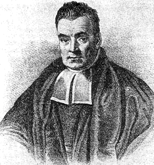
Note It is not clear whether this is actually a picture of him…

Bayesian

\[P(\text{Model}|\text{Data}) = \frac{P(\text{Data}|\text{Model})P(\text{Model})}{P(\text{Data})}\]

However, it can be simplified to

\[P(\text{Model}|\text{Data})\propto P(\text{Data}|\text{Model})P(\text{Model})\]

Estimating model parameters

Markov Chain Monte Carlo
Hamiltonian Monte Carlo
…

Our way of thinking is Bayesian

The different parts of a Bayesian model

\[\underbrace{P(\text{Model}|\text{Data})}_\text{Posterior}\propto \underbrace{P(\text{Data}|\text{Model})}_\text{Likelihood}\underbrace{P(\text{Model})}_\text{Prior}\]

When we look at the equation above, it might be difficult to visualize exactly what are the

Posterior
Likelihood
Prior

Understanding this will be essential for the course.

Let’s use a small example to make sure we understand each part of the Bayesian model well.

Illustrative example

For this example, we will be interested in building a model to study the breeding success of the kākāpō. The kākāpō (Strigops habroptilus) is a critically endangered large (fat!) flightless nocturnal parrot found solely on the islands of Whenua Hou, Pukenui and Te Kākahu-o-Tamatea in New-Zealand. There are currently only 236 adults kākāpō on Earth. So studying its breeding success can be very valuable for the survival of the species

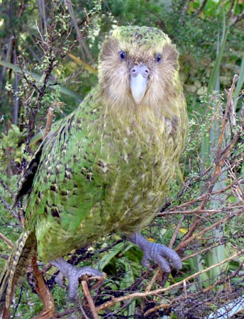
Sirocco Probably the most popular kākāpō.

If you wonder why Sirocco is popular, take a look at this YouTube video

Illustrative example

For the sake of this example, let’s focus on three female kākāpō, the number of eggs they laid and the number of chicks that hatched. Typically a kākāpō lay 1 to 4 eggs every breeding period, which occur every 2 to 4 years. In this example, we will assume we have data for the past 20 years (so, let’s assume we have data for the past 6 breeding period).

Kākāpō	Eggs laid	Chick hatched
Bella	12	4
Wendy	10	5
Nora	16	5

Note Kākāpō names and number of hatched chicks are real (see the List of kakapo), while number of laid eggs were invented but follow what is expected from current research.

Illustrative example

Based on the available information

Available data
Information provided
Assumptions we made

We can assume rely on the Binomial distribution in this example.

Do you know why ?

Illustrative example

Likelihood

What is the probability distribution that a kākāpō will produce chicks during the 20-year period?
\[ \begin{align} \text{chick hatched} &\sim \text{Binomial}(p, \text{eggs laid}) \\ \end{align} \]

This is the probability distribution associated to the kākāpō data.

It is called the likelihood.

Illustrative example

Likelihood

The likelihood is the product (\(\times\)) of the probabilities associated to each data point

\[L(\theta \mid x) = \prod_{i=1}^n P(x_i \mid \theta)\] where

\(P(x_i \mid \theta)\) is the function of a probability distribution function
\(x_i\) is the value associated to sample \(i\) out of \(n\) samples
\(\theta\) is the parameter associated to the model

In our example,

\(P(x_i \mid \theta)\) is the Binomial distribution function
\(x_i\) is the reproductive success of each kākāpō (\(i\)) over the 20 year period
\(\theta\) is the probability of reproductive success

Illustrative example

Likelihood

When writing the likelihood as

\[L(\theta \mid x) = \prod_{i=1}^n P(x_i \mid \theta)\]

we make the assumption that each observation, each sample is independent from all the other observations.

Later in this course, we will see how to work around this problem.

Illustrative example

Likelihood

We can thus write the likelihood conceptually as

\[ P(\text{Bella},\text{Wendy}, \text{Nora} \mid \theta) = P(\text{Bella} \mid \theta)\times P(\text{Wendy} \mid \theta)\times P(\text{Nora} \mid \theta) \]

and more formally as

\[ \begin{align*} P\left(4, 5, 5 \mid p\right) = &\text{Binomial}\left(4 | p, 12\right)\times \\ &\text{Binomial}\left(5 | p, 10\right)\times\\ &\text{Binomial}\left(5 | p, 16\right) \end{align*} \]

Illustrative example

Likelihood

Working directly with the likelihood is often problematic computationally because multiplication on probabilities can lead to technical problems

It is thus common to work with a log-likelihood function. In doing so, laws of logarithms allows us to convert multiplications to additions

\[ \begin{align*} \log\left(P\left(4, 5, 5 \mid p\right)\right) =& \log\left(\text{Binomial}\left(4 | p, 12\right)\right) + \\ & \log\left(\text{Binomial}\left(5 | p, 10\right)\right)+\\ & \log\left(\text{Binomial}\left(5 | p, 16\right)\right) \end{align*} \]

Illustrative example

Log-likelihood in R

# Data
hatch <- c(4, 5, 5)
eggs <- c(12, 10, 5)

# log-likelihood function
calc_ll <- function(x, 
                    hatch, eggs) {
  # Quick check
  if(length(hatch) != length(eggs)){
    stop("hatch and eggs must have the same length")
  }
  
  # log-likelihood
  res <- sum(-dbinom(hatch,
                     size = eggs,
                     prob = x,
                     log = TRUE))
  return(res)
}

# Test a range of probability values
prob_val <- seq(from = 0, 
                to = 1,
                length.out = 30)

# Result object
log_lik <- numeric(30L)

for (i in 1:length(prob_val)) {
  log_lik[i] <- calc_ll(prob_val[i],
                        hatch = hatch,
                        eggs = eggs)
}

par(cex = 3)
plot(prob_val,
     log_lik,
     type = "b",
     xlab = "Probability",
     ylab = "Log-likelihood")

Illustrative example

Let’s make it Bayesian

Add a prior

\[ \begin{align*} {P\left(4, 5, 5 \mid p \right)} = &\text{Binomial}\left(4 | p, 12\right)\times \\ &\text{Binomial}\left(5 | p, 10\right)\times\\ &\text{Binomial}\left(5 | p, 16\right)\\ p\sim & \text{Uniform}\left(\text{min}=0,\text{ max}=1\right) \end{align*} \]

Illustrative example

Let’s make it Bayesian

If we combine the likelihood and the prior we get

\[ \begin{align*} P\left(p \mid 4, 5, 5\right) =& \text{Binomial}\left(4 | p, 12\right) \times \\ & \text{Binomial}\left(5 | p, 10\right)\times\\ & \text{Binomial}\left(5 | p, 16\right)\times\\ & \text{Uniform}\left(\text{min}=0,\text{ max}=1\right) \end{align*} \]

Illustrative example

Let’s make it Bayesian

If we rewrite this model using logs we get

\[ \begin{align*} \log\left(P\left(p \mid 4, 5, 5\right)\right) =& \log\left(\text{Binomial}\left(4 | p, 12\right)\right) + \\ & \log\left(\text{Binomial}\left(5 | p, 10\right)\right)+\\ & \log\left(\text{Binomial}\left(5 | p, 16\right)\right)+\\ & \log\left(\text{Uniform}\left(\text{min}=0,\text{ max}=1\right)\right) \end{align*} \]

A few words about the prior

Definition of prior probability

The prior probability informes us about the probability of the model being true before considering any available data

Types of priors

“Uninformative”

These priors are meant to bring very little information to the model

Informative

These priors bring information to the model that is available

A few words about the prior

“Uninformative” priors

Example If we have no idea of how elevation influence sugar maple

Gaussian distribution

\[f(x)=\frac{1}{\sqrt{2\pi\sigma^2}}e^{-\frac{(x-\mu)^2}{2\sigma^2}}\]

\(\mu = 0\)

\(\sigma = \text{Large say 100}\)

A few words about the prior

Informative priors

Example If we know that

There are less sugar maples the higher we go
The influence of elevation on sugar maple cannot be more than two folds

Uniform distribution

\[f(x)=\left\{ \begin{array}{cl} \frac{1}{b-a} & \text{for } x\in [a,b]\\ 0 &\text{otherwise}\\ \end{array} \right.\]

\(a > -2\)

\(b < 0\)

Estimating Bayesian model

As I hinted earlier, there are a number of ways to estimate the parameters of a Bayesian model. A common way to estimate Bayesian models is to rely on Markov Chain Monte Carlo (MCMC) or variants of it, including Hamiltonian Monte Carlo (HMC), which is used in Stan.

Typical reasons to favour MCMC

It is flexible
It can be applied to complex models such as models with multiple levels of hierarchy

Why should we learn about MCMC ?

The goal of this course is not to learn the intricacies of MCMC or HMC, but since we will play a lot with Stan, it is important to learn at least conceptually how MCMC and HMC work.

Markov Chain Monte Carlo (MCMC)

Historically, the developments of MCMC have been intimately linked with the arrival of computers. Specifically, the first developments and applications of MCMC were made in the early 1950’s at the Los Alamos laboratory.

MANIAC I is The first computer on which MCMC was implemented

Markov Chain Monte Carlo (MCMC)

A key figure in the development of MCMC was Arianna W. Rosenbluth, who was the first to implement an MCMC.

Arianna W. Rosenbluth (1927 - 2020)

Markov Chain Monte Carlo (MCMC)

To explain what is an MCMC, let’s imagine that we are interested in understanding how the mallard (Anas platyrhynchos) grows from hatchling to adult.

Markov Chain Monte Carlo (MCMC)

A simplistic statistical example

Let’s say that we are interested in modelling how male Mallard weight changes as they grow from hatching to adult. Here are some data obtained from a local Mallard duck farm.

Markov Chain Monte Carlo (MCMC)

A simplistic statistical example

A growth model can be constructed using a simple linear regression

\[y = \beta_0 + \beta x + \varepsilon\] From this model we can infer that the average weight of a Mallard duck when it hatches is 107 grams (intercept), and the average daily growth of the Mallard is 13.5 grams (slope).

Markov Chain Monte Carlo (MCMC)

A simplistic statistical example

Estimating the intercept and slope parameters of the simple linear regression can be done with an MCMC. This amount to sampling

\(\beta_0\) as

\[\beta_0 \sim \mathcal{D}(\text{mean}, \text{variance}, \text{skewness}, \text{kurtosis}, \dots)\]

and \(\beta\) as

\[\beta \sim \mathcal{D}(\text{mean}, \text{variance}, \text{skewness}, \text{kurtosis}, \dots)\]

In doing so, we are not focusing on finding the ‘best’ parameter values. Rather, we are focused on finding the distribution of best parameter values.

Markov Chain Monte Carlo (MCMC)

When using an MCMC, we are interested in sampling distributions to estimate the parameters of the model.

Technically, MCMC and HMC rely on different approaches to assess the structure of the distributions.

Markov Chain Monte Carlo (MCMC)

MCMC relies on using many random samples to assess the structure of the distribution.

Markov Chain Monte Carlo (MCMC)

Problems with Markov Chain Monte Carlo

A lot of tuning is required to find the best step length (between long and short steps)
Inefficient in high-dimensional spaces
Cannot easily search the entire likelihood space and thus cannot easily isolate local minima

Hamiltonian Monte Carlo

Hamiltonial Monte Carlo relies on Hamiltonian dynamics to assess the structure of the distribution.

Hamiltonian Monte Carlo

Solution brought by Hamiltonian Monte Carlo

Uses a gradient-based MCMC to reduce the random walk (hence reduce autocorrelation)
It is a “No-U-Turn Sampler” (NUTS)

If you do not fully get it (and even if you do), check out the Brilliantly wrong

Sampling the parameters

In MCMC and HMC, a lot of iterations need to be carried out to assess the distribution of parameters. But how many is enough ?

Here is a rough procedure to follow:

Perform a pilot run with a reduced number of iterations (e.g. 10) and measure the time it takes
Decide on a number of steps to use to obtain a result in a reasonable amount of time
Run the algorithm again !
Study the chain visually

Studying convergence

If we ran the same MCMC as above but instead for 50000 steps, we obtain

Note It is also possible to thin (record only the \(n^{\text{th}}\) iteration), but it is better to keep all iterations when possible. Actually, thinning should only be carried out when there are too many iterations for you to keep them on your computer and manipulate them. In short, thinning should be carried out only when your computer does not have enough memory to work with all iterations.