Maximum likelihood

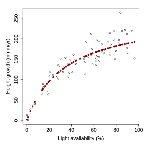
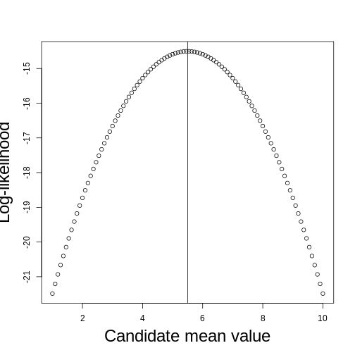
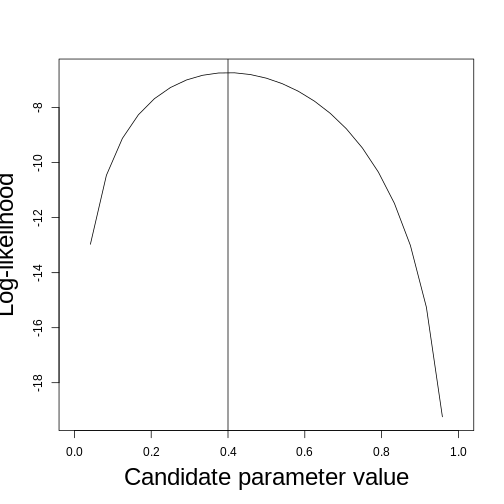
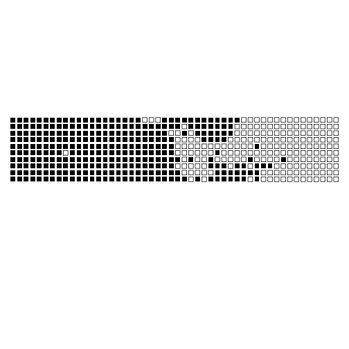
class: title-slide, middle

# Model evaluation with ecological data

## Maximum likelihood

.instructors[
  **ECL707/807** - Dominique Gravel
]

---

# Go back to hemlock's growth

![](07_likelihood_files/figure-html/unnamed-chunk-1-1.png)

How do you propose to evaluate model fit ?

---

# A standard statistical model

`$$y_i = \alpha + \beta x_i + \epsilon_i$$`

with

`$$\epsilon \backsim \eta(0,\sigma^2)$$`

where `$\alpha$`, `$\beta$` and `$\sigma$` are fitted parameters.

---

# Another way of formulating a statistical model

`$$y \backsim \eta(\mu, \sigma^2)$$`

where

`$$\mu_i = \alpha + \beta x_i$$`

In other words, this means that the probability of an observation `$data_i$` is distributed as `$P(y = data_i|x_i, \alpha, \beta, \sigma)$`

---

# Deeper in the inference philosophies

*Example from Bolker (2009) chapter 1)*

## Seed predation

Data quantifies how many times the seeds from a small-seed species (*Polyscias fulva*) and a large-seed species (*Pseudospondias microcarpa*) are predated in an experiment in Kibale National Park, Uganda.

Data looks like :

|              | Small | Large |
|--------------|-------|-------|
| Predation    | 26    | 25    |
| No predation | 184   | 706   |
| Total        | 210   | 731   |

---

# Classical frequentist

- Calculate the parameter of a particular phenomenon, here the frequency of predation
- Calculate a p-value defined as **the probability of that outcome given a specified null hypothesis**
- Reject this null hypothesis if the p-value is below a threshold; don't accept the null if it is large, just fail to reject it

---

# Classical frequentist
## Seed predation

Proportion of seeds are predated are respectively `$26/210 = 0.124$` and `$25/731 = 0.034$`, which means that predation rate being `$0.124/0.034 = 3.62$` larger for the small seed species.

Are these rates different ? Or more precisely in a frequentist way, what proportion of possible outcomes would result in observed ratios greater than `$3.62$` if the two predation rates were the same ?

Fisher's exact test yields the probability `$p=5.26x10^{-6}$`. This number represents the strength of evidence against the null hypothesis (which is often interpreted as the strength of evidence in favor of the alternative hypothesis).

---

# Likelihood

The maximum likelihood approach finds the set of parameters (here the seed predation rates) that makes the observed data the most likely to have occurred. The challenge is to find the model and associated parameters that are the most likely given the observations.

Note that it is possible to add a *frequentist* interpretation to a maximum likelihood analysis. For instance, one could compute confidence intervals around parameters and test for a null hypothesis. Another approach is to compare the likelihood of an alternative hypothesis to the likelihood of a null hypothesis and set up a cutoff criteria to take a decision. 
---

# Likelihood
## How to do it

The number of seeds that are predated is binomially distributed with associated probabilities `$p_{small} = 0.12$` and `$p_{large}=0.034$`. No need to go into the full proof (see Clark (2009) for the derivation) to show these probabilities are maximum likelihood estimates (MLE).

We use the binomial distribution to get the probability of the data given these parameters, which are respectively `$P(\theta_{small}|data) = 0.083$` and `$P(\theta_{large}|data) = 0.081$`. The likelihood of the whole dataset, given these parameters is `$0.081$`.

We do the same for the overall predation rate ($51$ seeds out of `$941$` trials) and obtain `$P(\theta_{all}|data) = 0.057$`.

We conclude from these numbers that different predation rates are more likely to generate the observations than a single predation rate.

---

# Bayesian

Frequentist statistics assume there is a *single truth* to reality given rise to the distribution of experimental outcomes. Bayesian statistics say instead the the experimental outcome is the truth, while the parameter values do have a distribution.

The strength of the bayesian framework is that we can legitimately make statements about the probability of different hypotheses.

As a complement, it requires to specify *prior belief* to derive the *posterior* distribution of hypotheses.

---

# Bayesian 
## Shortcut solution

We will say that the posterior distribution of predation rates will follow the function :

`$$P(\theta_{small}|data) \propto P(data|\theta_{small})P(\theta_{small})$$`

Fow which we could compute the mode (the value of `$\theta$` where the posterior distribution reaches its peak). Doing it requires defining the prior distribution `$P(\theta_{small})$` and a bit of algebra. In some instances we have no clue and will specify a non-informative prior (here a flat beta distribution), in other situations we may do include previous knowledge (e.g. another experiment). Then after parameter distributions are compared.

The conclusion will be a probability statement on the occurrence of the alternative hypothesis, here that the rates are different (skipping the details, the answer is that the posterior probabiilty that predation rates differ is `$0.996$`).

---
class: inverse, middle, center

# Where do you find yourself ?

---

# The "likelihood principle"

`$$\zeta (\theta|data) \propto P(data|\theta)$$`

In words: The likelihood ( `$\zeta$` ) of the set of parameters ( `$\theta$` ) (in the scientific model), given an observation ( `$data$` ), is proportional to the probability of observing the data  given the parameters...

The likelihood approach flips the interpretation of a statistical model : the data is the reality, and we look at the "likelihood" of an explanation. Among several things, this formulation facilitates the comparison of candidate models (and sets of parameters).

---

# Likelihood for a set of observations

The likelihood of a set of observation is the joint probability of the different data points given the model. Using product rule, for `$i = 1...n$` independent observations, and a vector of `$\mathbf{X}$` observations ( `$x_i$` ), we obtain :

`$$\zeta (\theta|\mathbf{X}) \propto \prod g(x_i|\theta)$$`

A product of probabilities is a very small number, so often we prefer to use logarithms, such that the log-likelihood is :

`$$log[\zeta (\theta|\mathbf{X})] \propto \sum log[g(x_i|\theta)]$$`

---

# A very basic example

**Estimating the mean of a set of values**

Let consider the following set of numbers `$X = \{4, 2, 10, 5, 8, 4\}$`. It's very straightforward to compute the mean, but how to do it by maximum likelihood ?

---

# Routine for finding best parameters

```
DEFINE probability distribution

REPEAT
  PROPOSE parameters
  EVALUATE likelihood of every observation
  SUM the log likelihood
  COMPARE to previous solution
  RECORD solution if it improves log-likelihood
UNTIL no further improvement

```

---

# A very basic example

**Estimating the mean of a set of values**

Let's try first by minimizing the sum of squares as we do with traditional linear models :

```r
ss <- function(X, u) {
  res <- (X-u)*(X-u)
	return(sum(res))
}
X <- c(4, 2, 10, 5, 8, 4)
ss(X, 5)
```

```
## [1] 45
```

```r
ss(X, 5.5)
```

```
## [1] 43.5
```

---

# A very basic example

Now let's do it by maximizing the likelihood, assuming a normal distribution of residuals :

```r
ll <- function(X, u, sd) {
	sum(dnorm(X, u, sd, log = TRUE))
}
ll(X, 5, 1)
```

```
## [1] -28.01363
```

```r
ll(X, 5.5, 1)
```

```
## [1] -27.26363
```

```r
ll(X, 5.5, 2.95)
```

```
## [1] -14.50374
```

---

# A very basic example
## Likelihood profile / surface
 
![](07_likelihood_files/figure-html/unnamed-chunk-4-1.png)

---

# A different approach to inference

*We believe that “truth” (full reality) in the biological sciences has essentially infinite dimension, and hence ... cannot be revealed with only ... finite data and a “model” of those data...*

*... We can only hope to identify a model that provides a good approximation to the data available.*

Burnham and Anderson 2002, p. 20

---

# Exercise 2.1. 
## Time to sharpen your pen...

I want to estimate the probability that the bee *Bembix oculata* visits the flower *Mentha pulegium* over a sampling time of 5 minutes. I do 10 transects, in which I record for each of them if an individual visits a flower and obtain the following sequence of events `$X = \{0, 1, 1, 0, 1, 1, 0, 0, 0, 0\}$` representing if an interaction occurred ( `$X_i = 1$` ). What is the maximum likelihood estimate for this dataset ?

---

# Solution 2.1.

What we aim to describe is a binomial process with 10 trials. We seek to estimate the interaction probability `$p$`.

If we observe an interaction, the likelihood of that event is `$p$`, while if we do not observe the interaction the likelihood is `$1-p$`.

As a result, we get the following likelihood for each observation `$L = \{1-p, p, p, 1-p, p, p, 1-p, 1-p, 1-p, 1-p\}$`.

---

# Solution 2.1.

We simply have to sum the log of these values and find the `$p$` that maximizes this number.

![](07_likelihood_files/figure-html/unnamed-chunk-5-1.png)

---
class: inverse, middle, center

# Step by step guide to compute the likelihood of your data given your model

---

# Recall : Another way of formulating a statistical model

Data (your observations) are distributed according to a *probability function*

`$$y \backsim \eta(\mu, \sigma^2)$$`

where the *scientific model* is

`$$\mu_i = \alpha + \beta x_i$$`

And accordingly, your objective is to compute :

`$$P(y = data_i|x_i, \alpha, \beta, \sigma)$$`

The *likelihood function* that you have to code is the function for `$P(data|covariates, parameters)$`

---

# Step 0 (an old C++ habit ...)

Conceptual part. By far the most important, often the one that we neglect. Impossible to go forward with the R code if this part is not clear. This should all be done with paper and pen.

- What is the data you want to predict. Name it (e.g. **obs** or **Y**)
- Are there covariates ? Name them (e.g. **X** or **elevation**)
- Identify the proability function (PDF or PMF)
- Identify parameters of the probability function 
- Propose an equation for your scientific model 
- Make sure that you understand how to plug the result of your scientific model into the probability functions (e.g. how is the mean changing with the covariates)
- Write all of this on paper

---

# Step 1

Propose candidate values for all parameters

---

# Step 2

Write the equation to compute the model prediction for each observation of covariates (ie sampling unit) given the proposed parameters and the equation you wrote before. Call these numbers **pred**.

---

# Step 3

Use a probability function (e.g. dnorm) to compute the probability of each observation (data point).

This is straightforward with **dnorm** because the mean argument is your **pred**. But it may be more complicated for other PDFs because the parameters are not necessarily corresponding to the mean, e.g. beta or gamma. In some instances you don't even have a PDF (e.g. the logistic regression where the scientific model is the PDF at the same time).

---

# Step 4

Take the log of all probabilities and sum it. This is your log likelihood !

---

# Step 5

Repeat steps 1-5 until you believe you found the paramaters that maximize your likelihood.

**Note:** You may want to wrap steps 2-4 into a function because you will have to repeat these steps often.

---

# Summary : pseudo-code of a likelihood function

```
DRAW parameters

DEFINE model(covariates, parameters)
DEFINE pdf(obs, predict, parameters)

COMPUTE pred <- model(covariate, parameters) 
COMPUTE p_obs <- pdf(obs, pred, parameters)
COMPUTE ll <- sum(log(p_obs))
```
---

# Exercise 2.2. 
## Time to practice : maple distribution at Sutton

![](07_likelihood_files/figure-html/unnamed-chunk-6-1.png)

---

# Exercise 2.2.
## A species distribution problem

**The model**

`$$y \thicksim f(E, \theta)$$`

- f is a probability density function
- `$y$` is the abundance (in stems per quadrat) of sugar maple
- `$E$` is elevation
- `$\theta$` is a set of parameters

**Things to think about :** 
- What are the characteristics of the data ? 
- What is the form of the function ? 
- What is the probability density function ?

---

# Exercise 2.2.
## Try first a linear regression

How does it look ? What's the problem ?

---

# Exercise 2.2.
## Logistic regression

And now what's the problem ?

---

# Exercise 2.2.
## A non-linear function

Do we have the appropriate PDF ?

---

# Exercise 2.2.
## A poisson PDF

---

# Useful distributions to get familiar with

**For discrete events:**

- Binomial
- Multinomial
- Poisson
- Negative binomial

**For continuous events:**

- Normal
- Lognormal
- Gamma
- Beta

---

# How to choose the right one

- Type of data 
- Is the data bounded ?
- Look at the residuals
- Hypothesis / theory driven

---

# Typical problems with likelihood evalution

- Log of null or negative probabilities
- Likelihood functions converging to 0 in the limit of `$\theta \rightarrow \infty$`
- Numerical errors (e.g. a normal distribution with a very small SD)
- Impossible predictions (e.g. negative probabilities)
- Underflow / Overflow (if you forget to log)
- Very rough likelihood surface

---

# Finding the optimal solution

Next lecture !