The Simulated Annealing Algorithm, 2 ways

Dom’s Solution

# Load the data 
data <- read.table("data/hemlock.txt", header = TRUE)
obs = data[,2]
L = data[,1]

# Likelihood function
h <- function(obs, L, pars) {
    a <- pars[1]
    s <- pars[2]
    sigma <- pars[3]
    mu <- a*L/(a/s + L)
    sum(log(dnorm(obs, mu, sigma)))
}

# Candidate function
c_x <- function(pars_lo, pars_hi) runif(1, pars_lo, pars_hi)

# Set conditions for the simulated annealing sequence
T_fn <- function(T0, alpha, step) T0*exp(alpha*step)

T0 <- 10
alpha = -0.001
nsteps <- 10000

# Prepare an object to store the result
res <- matrix(nr = nsteps, nc = 5)

# Initiate the algorithm
a0 <- 1
s0 <- 1000
sd0 <- 10
pars0 <- c(1, 100, 10)
pars_lo <- c(0, 1, 1)
pars_hi <- c(1000, 1000, 100)

# Main loop
for(step in 1:nsteps) {

    for(j in 1:3) {

        # Draw new value for parameter j
        pars1 <- pars0
        pars1[j] <- c_x(pars_lo[j], pars_hi[j])

        # Evaluate the function
        h1 <- h(obs, L, pars1)
        h0 <- h(obs, L, pars0)

        # Compute the difference
        diff <- h1 - h0

        # Accept if improvement
        if(diff > 0) pars0 <- pars1

        # Accept wrong candidates 
        else {  
            p <- exp(diff/T_fn(T0, alpha, step))
            if(runif(1)<p) pars0 <- pars1
        }
    }
    
    # Record values
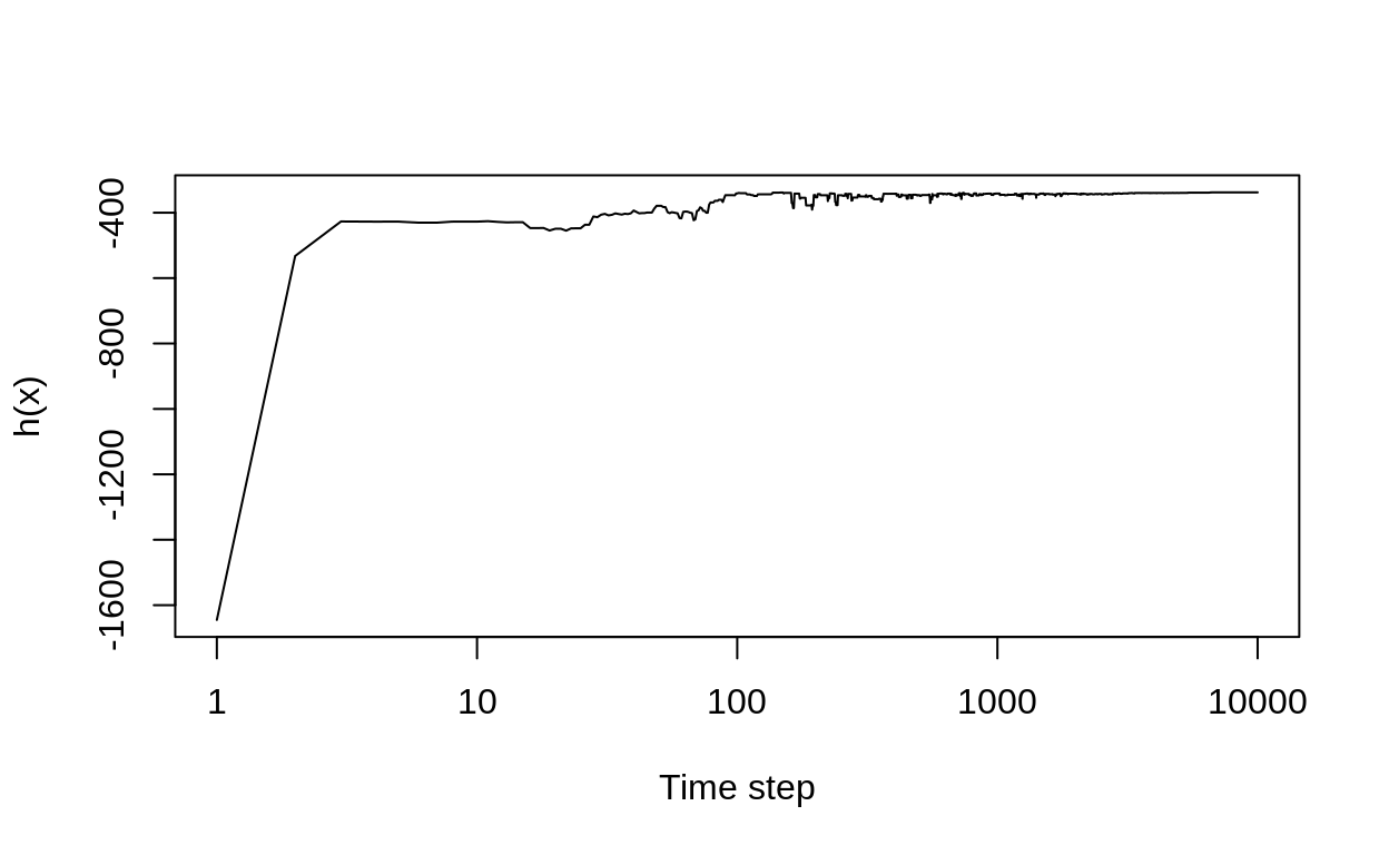
    res[step,] <- c(step,pars0,h(obs,L,pars0)) 
}

#Plot the results
plot(c(1:nsteps), res[,5], type = "l", xlab = "Time step", ylab = "h(x)",cex = 2, log = "x")

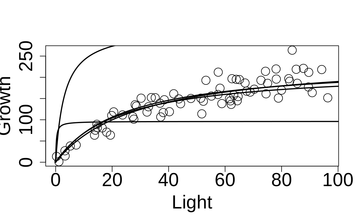
plot(L, obs, cex = 2, xlab="Light", ylab = "Growth", cex.axis = 2, cex.lab = 2)

add_model<- function(step) {
    Lseq = seq(0,100,0.1)
    a=res[step,2]
    s=res[step,3]
    lines(Lseq,a*Lseq/(a/s+Lseq), lwd = 2)
}
add_model(2)
add_model(10)
add_model(100)
add_model(500)
add_model(1000)

Andrew’s Approach

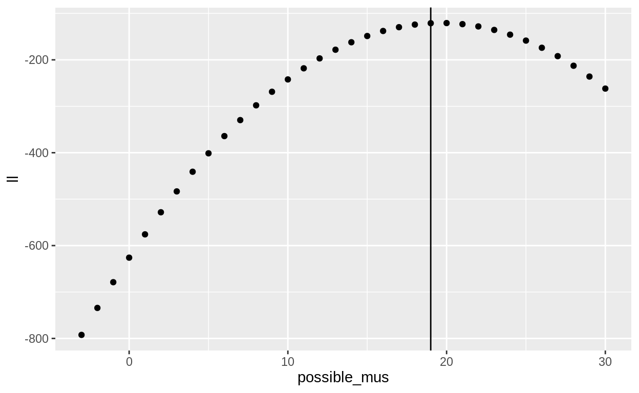
Rather than using the hemlock data, this example uses 42 random numbers, and tries to identify the known mean of 19.

DEFINE function to optimize h(X)

set.seed(1316)

fake_xs <- rnorm(42, 19, 4)

loglike_numbers <- function(numbers, mu) sum(dnorm(x = numbers, mean = mu, sd = 4, log = TRUE))


loglike_numbers(fake_xs, 7)

[1] -329.7753

library(tidyverse)

tibble(possible_mus = -3:30) %>% 
  mutate(ll = map_dbl(possible_mus, loglike_numbers, numbers = fake_xs)) %>% 
  ggplot(aes(x = possible_mus, y = ll)) + geom_point() + 
  geom_vline(xintercept = 19)

DEFINE the sampling function c(X)

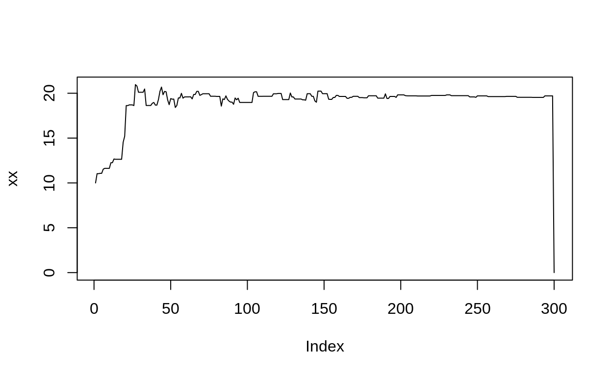
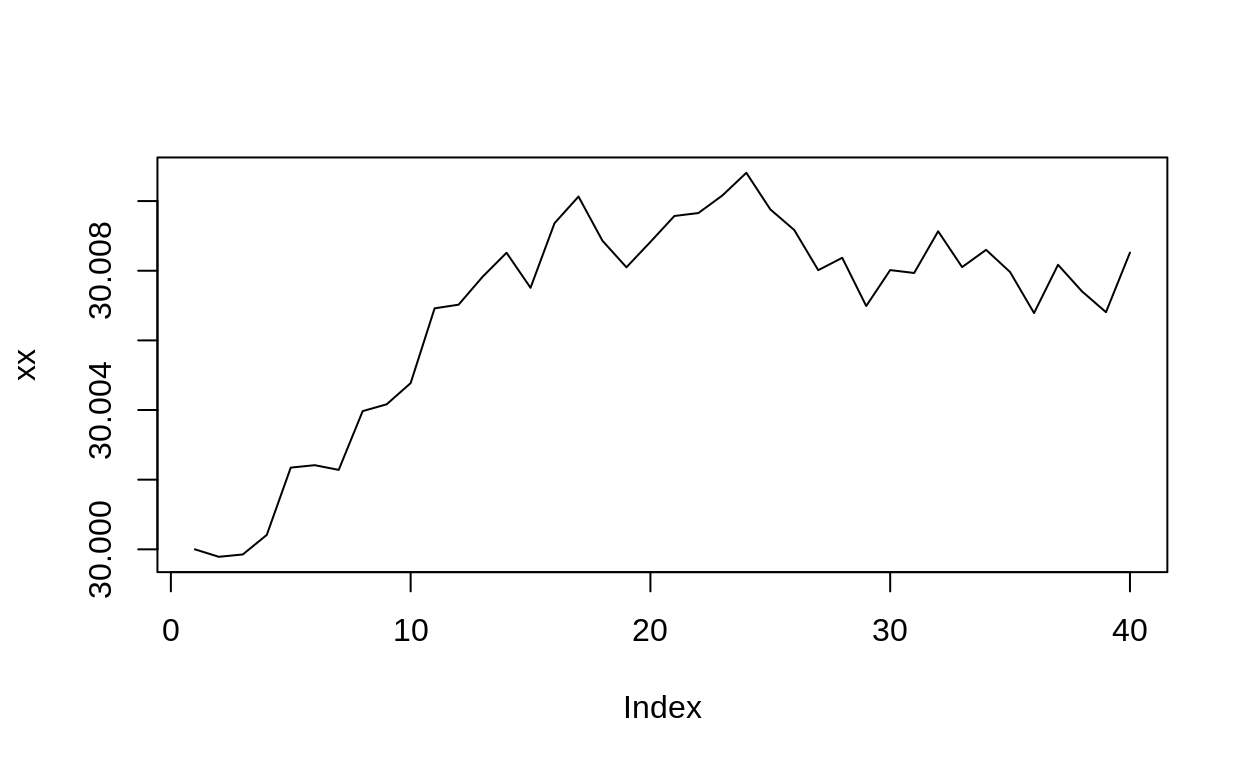
see_of_x <- function(x, sigma = 1) { x + rnorm(1, sd = sigma) }

xx <- numeric(40)
xx[1] <- 30

## walk like a drunk: test my see of x function
for(i in 2:40){
  xx[i] <- see_of_x(xx[i-1], sigma = .001)
}

plot(xx, type = "l")

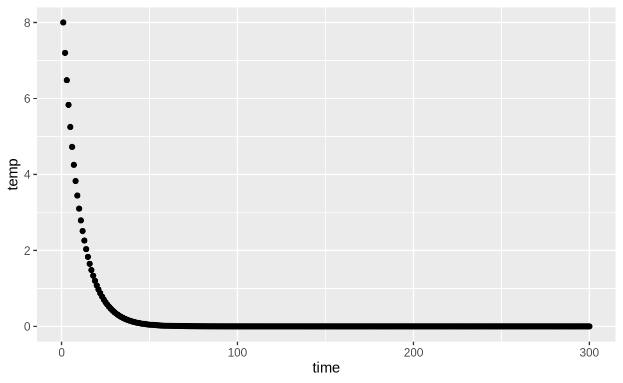
DEFINE temperature sequence

temp_line <- function(runs, tstart, tcool){
  exp(log(tstart) + log(tcool)*0:(runs-1))
}

temp_line_str <- function(runs, tstart) {
  seq(tstart, 0, length.out = runs)
}

tibble(time = 1:300,
       temp = temp_line(300, 8, 0.9)) %>% 
  ggplot(aes(x = time, y = temp)) + 
  geom_point()

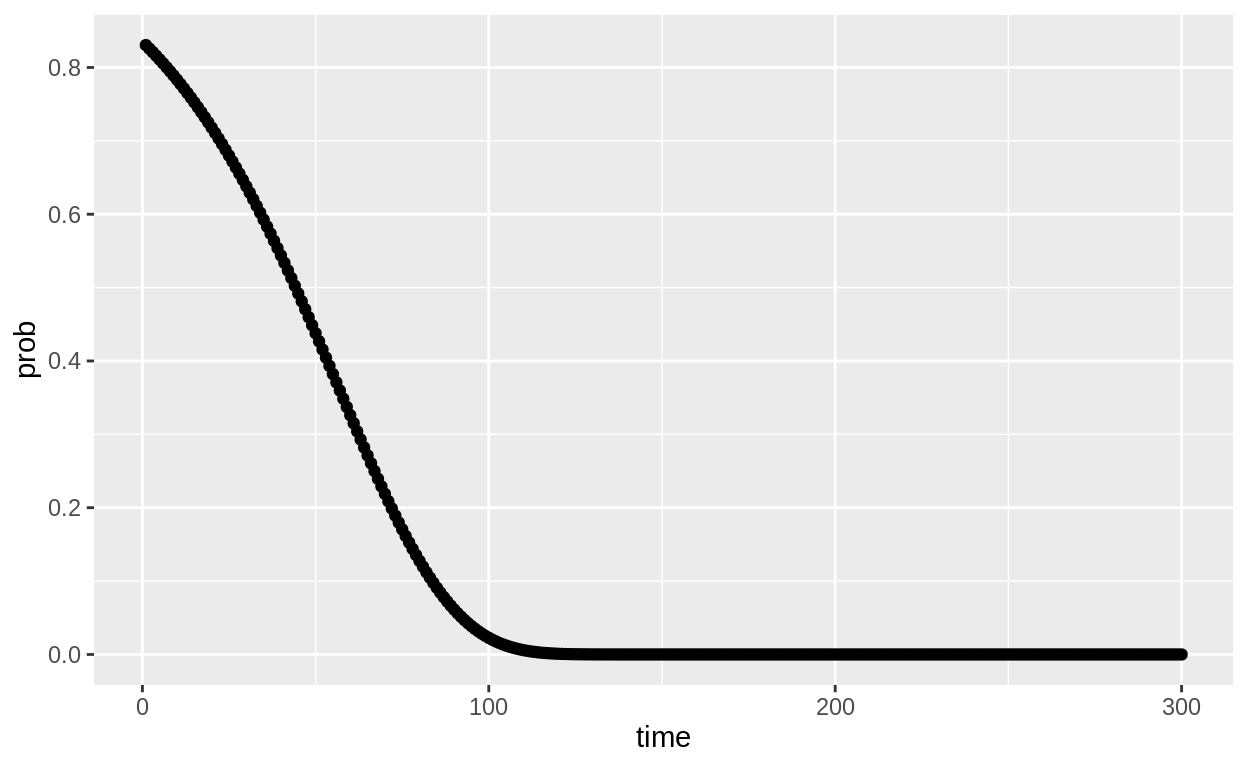
tibble(time = 1:300,
       prob = exp(-13/temp_line(300, 70, 0.97))) %>% 
  ggplot(aes(x = time, y = prob)) + 
  geom_point()

    REPEAT
        DRAW sample X from c(x)
        COMPUTE difference diff = h(X) - h(X_0)
        IF diff > 0 ACCEPT X
        ELSE 
            COMPUTE acceptance probability p = exp(diff/T)
            DRAW value P from random uniform on (0,1)
            IF P < p
                ACCEPT X
            ELSE
                REJECT X
        UPDATE temperature
    UNTIL nsteps is reached

# function to take temperature, diff, and give back TRUE or FALSE (will a negative be kept)

keep_neg_diff <- function(diff, Tmp){
  stopifnot(diff<0)
  runif(1, min = 0, max = 1) < exp(diff/Tmp)
}

keep_neg_diff(-30, Tmp = 40)

[1] FALSE

keep_neg_diff(10, Tmp = 0)

Error in keep_neg_diff(10, Tmp = 0): diff < 0 is not TRUE

## function to take x0 and x1 and a function and temp and return either x0 (reject) or x1 ( accept)
keep_or_reject <- function(x0, x1, fun, temp){
  diff <- fun(x1) - fun(x0)
  # browser()
  if (diff > 0) {
    return(x1)
  } else if (keep_neg_diff(diff, Tmp = temp)){
    return(x1)
  } else {
    return(x0)
  }
}

# evaluate for these only

ll_fakenums_f_x <- function(x) loglike_numbers(fake_xs, mu = x)

# make temperatures
runs <- 299

temps <- temp_line(runs, 3, 0.98)

xx <- numeric(runs + 1)

startval <- 10


xx[1] <- startval


for (i in 2:runs){
  maybe <- see_of_x(xx[i-1])
  xx[i] <- keep_or_reject(x0 = xx[i-1], x1 = maybe, fun = ll_fakenums_f_x, temp = temps[i-1])
}

plot(xx, type = "l")