Grid Search in the tidyverse

x_obs <- rbinom(10, 6, 0.6)
x_obs

 [1] 2 3 6 3 4 4 4 6 4 4

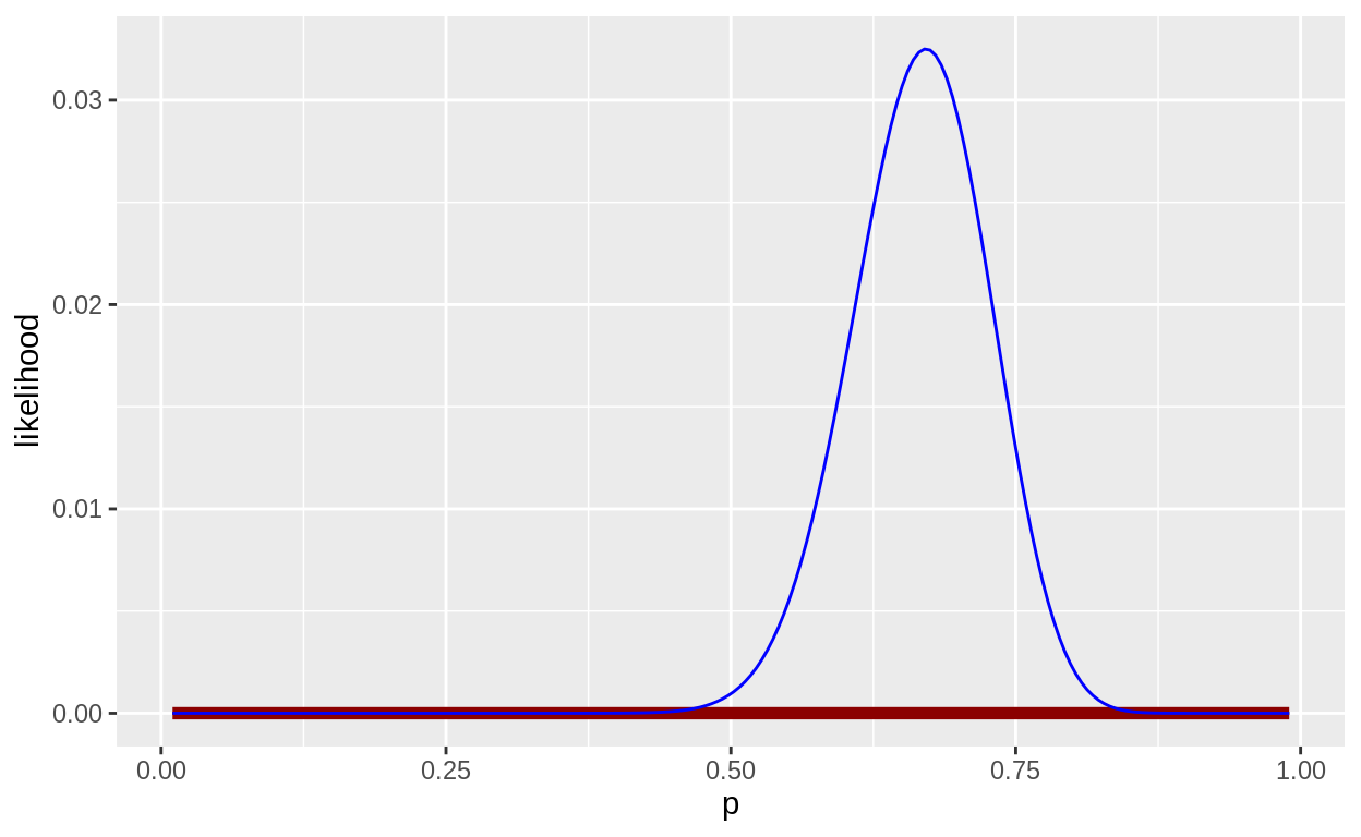
like_binom <- function(p, d = x_obs){
  exp(sum(dbinom(d, size = 6, prob = p, log = TRUE)))
}


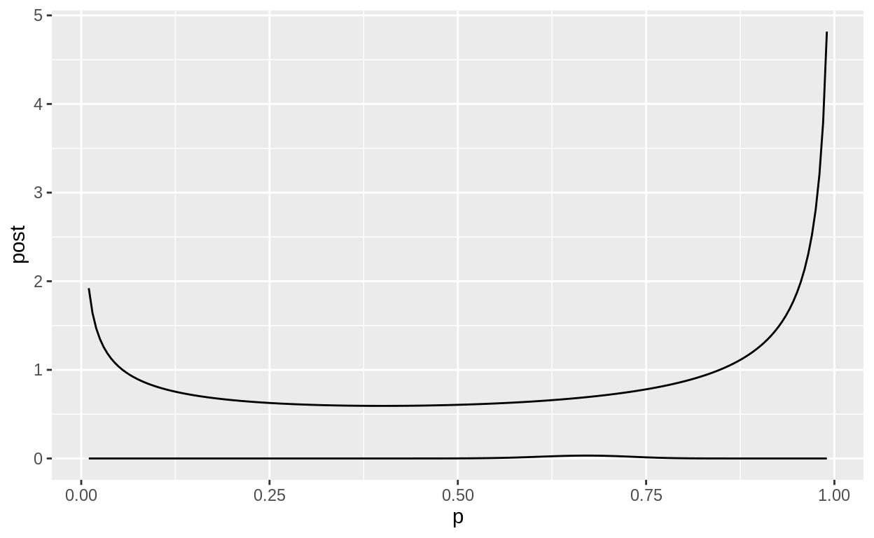
grid_searched <- tibble::tibble(
  p = seq(from = 0.01, to = .99, length.out = 200),
  density_p = dbeta(p, .03*20, (1-.03*20)),
  likelihood = purrr::map_dbl(p, like_binom),
  prior_times_likelihood = density_p * likelihood,
  post = prior_times_likelihood / sum (prior_times_likelihood)
)

head(grid_searched$likelihood)

[1] 3.726588e-71 3.048820e-64 2.478711e-59 1.586601e-55 2.023568e-52
[6] 8.456512e-50

library(ggplot2)
ggplot(grid_searched, aes(x = p, y = likelihood)) +
  geom_line() +
  geom_line(aes(y = prior_times_likelihood), lwd = 2, col = "darkred")  +
  geom_line(aes(y = post), col = "blue")

ggplot(grid_searched, aes(x = p, y = post)) + geom_line() +
  geom_line(aes(y = density_p))

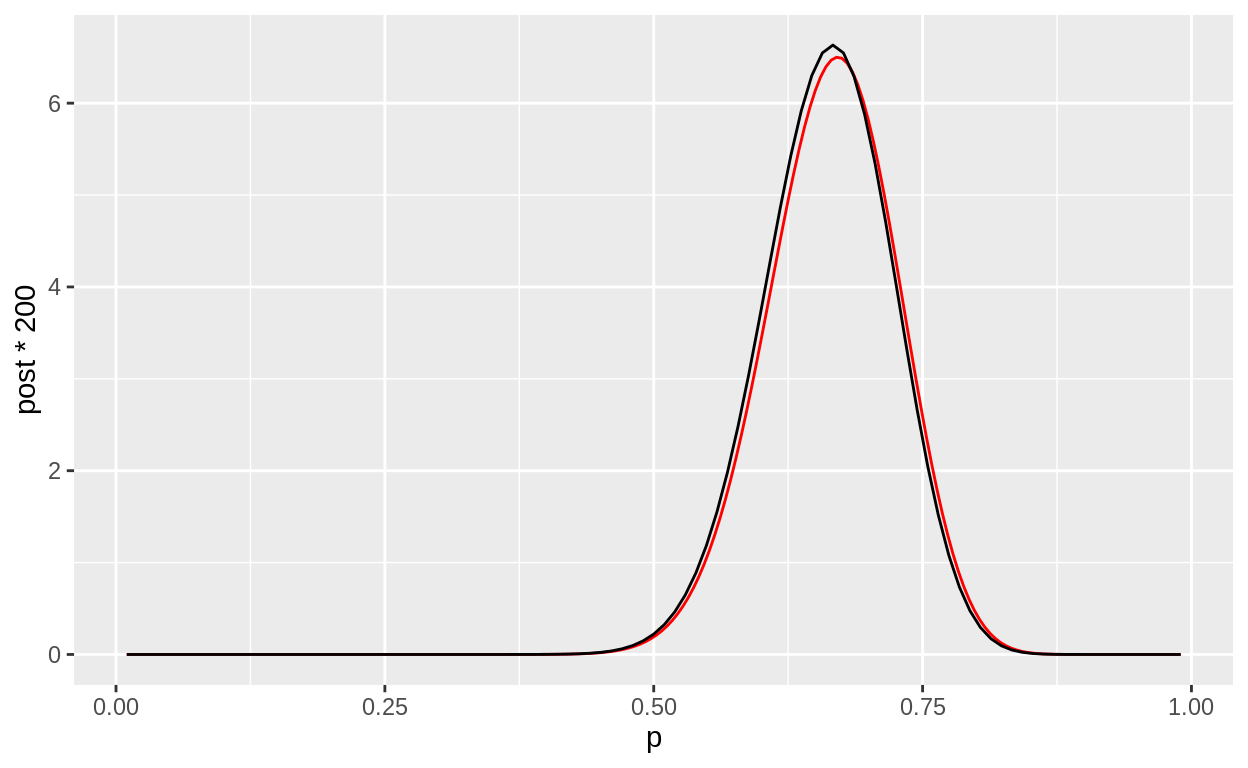
# calculate conjugate posterior
## prior  = dbeta(1, 1)
## posterior
# dbeta(x, 1 + sum(xobs), 1 + sum(6 - xobs))


ggplot(grid_searched, aes(x = p, y = post*200)) +
  geom_line(col = "red") +
  stat_function(fun = function(x) dbeta(x,
                                        1 + sum(x_obs),
                                        1 + sum(6 - x_obs)))