Why we do what we do

In bayesian statistics we use probability distributions to measure uncertainty about the parameter values we care about.

Because we measure uncertainty with probability, that means we work in probability distributions. We begin with distributions, and we end with distributions. The beginning distributions express all we want to say about what our parameters are. They come first, and are called the “prior” distributions. After we collect data and apply some model to relate it, we find ourselves with a new set of distributions. Because these come after the process of data collection and model creation, this is called the “posterior”.

This means we are applying Bayes rule. This shows us how to update our priors to reflect what we learned from the experiment and model building:

\[ \begin{align} [\theta_1, \theta_2 | \bf y] &\propto [\theta_1, \theta_2, \bf y] \\ &\propto [\bf y | \theta_1, \theta_2][\theta_1][\theta_2] \\ \end{align} \]

Refreshing questions:

which of these is the likelihood? Which is the prior?
why is it OK to use something proportional to (\(\propto\)) what we want?

The whole goal here is to get this posterior distribution. There are many ways to do this! This workshop is about some of them.

Conjugate priors – works for 1-parameter problems. Gives you the literal equation of the posterior distribution. Only directly useful for very simple problems. Becomes the absolute star of the show with Gibbs Sampling.
Laplace Approximation – very handy, useful best guess for many multi-parameter models; we’re not doing it.
Metropolis – A venerable classic for sampling simple models. You have to propose random “jumps” around the distribution, and these need to be symmetric
Metropolis-Hastings – same as Metropolis, but the jumps get to be asymmetric.
Gibbs sampling – A wonderful technique for simplifying complex problems. Requires that priors be chosen to make conjugate pairs with likelihoods.
Metropolis-in-Gibbs – is a Deluxe Combo of the previous two.
HMC etc – Hamiltonian Monte Carlo is an advanced modern way of doing the same thing. Sets you free to use the priors that work for your question, not the ones that work for your math.

MCMC in general

The objective of MCMC algorithm is to sample parameters from a complex posterior distribution.

Rather than measure the absolute probability of different parameter values:

\[ [\theta|y] = \frac{[y|\theta][\theta]}{[y]} \]

we sample, and evaluate the relative probability of two possible parameter values:

\[ \frac{[\theta^{new}|y]}{[\theta^k|y]} = \frac{[y|\theta^{new}][\theta^{new}]}{[y|\theta^k][\theta^k]} \]

In this way, we can sample a probability distribution ( \([\theta|y]\) ) using only something proportional to that distribution ( \([y|\theta][\theta]\) ). Put another way, we can’t get an equation, so we use interesting numerical tricks to jump straight to a histogram.

The Metropolis Algorithm

STEP 1 Draw \(\theta^{new}\) from a symmetric distribution centered on \(\theta^{k}\) (i.e. in the \(k\)th interation, the current value) e.g. \(\theta^{new} \sim N(\theta^{k}, \sigma_{tune})\)

STEP 2 Calculate the ratio R:

\[ R = \text{min}\left( 1, \frac{[y|\theta^{new}][\theta^{new}]}{[y|\theta^k][\theta^k]}\right) \]

This is the probability of acceptance. In other words, if the ratio is greater than one, that means the proposal is for a more probable value. We’ll always take it. If the ratio is less than 1, that means the new proposal is less probable than the value we have already. However, there’s a chance we’ll take it anyway.

STEP 3 Test to see if runif(1, min=0, max=1) \(< R\). if so, set \(\theta^{k + 1} = \theta^{new}\)

Why should we accept “worse” parameter values? Why is it good to sometimes stay in the same place?

Metropolis demo: the mean of the Normal Distribution

Let’s simulate some data from a normal distribution.

set.seed(1859)
M_true_mean <- 50
correct_sd <- 3
weights <- rnorm(300, mean = M_true_mean, sd = correct_sd)

head(weights)

[1] 48.23651 45.77398 48.84943 47.19116 50.31188 52.54827

One possible model for these data could be:

\[ \begin{align} y &\sim \text{Normal}(\mu, 3) \\ \mu &\sim \text{Normal(40, 10)} \end{align} \]

NOTE: We assume we KNOW the standard deviation. In this case, it is exactly 3. This is just for illustration. Later we will see what to do if you have multiple parameters.

To set up a Metropolis sampler, we’ll start by defining four useful functions:

A function which returns the log-likelihood of our data. As you recall, the likelihood of one datapoint is the probability of sampling that datapoint from a distribution, given specific known parameters. The likelihood of the data is the probability of observing ALL the datapoints. We assume the observations are independent, so we multiply the probability of each datapoint to get the probability of the whole dataset. Because we’re working on the log scale, instead of multiplication we just use addition.
a proposal function. This makes new values to try at each iteration of the Markov Chain. Here we’ll use a symmetric proposal function, the uniform distribution.
A convenience function to add the log-likelihood and the prior together – this gives us the numerator of the Bayes formula.
finally, a function which puts it all together and spits out the probability of acceptance. Because this is a probability, we use exp() to convert from log-likelihood values back to probability.

## define likelihoods for our problem
MEAN_normal_loglike <- function(data_vec, mean_value){
  sum(dnorm(data_vec, mean = mean_value, sd = 3, log = TRUE))
}

# proposal function to make new parameter values.
M_propose_new_val <- function(old_value, tune) {
  runif(1, min = old_value - tune, max = old_value + tune)
}

## function to use these to calculate the value of the numerator in Bayes Formula
## We are working on the LOG scale, so we have to ADD these together
numerator <- function(value, data)  {
  # likelihood
  log_like <- MEAN_normal_loglike(data_vec = data, mean_value = value)
  # prior
  log_prior <- dnorm(x = value, mean = 40, sd = 10, log = TRUE)
  
  return(log_like + log_prior)
}

## function to calculate the acceptance ratio
M_accept_probability <- function(new_value, 
                               old_value, 
                               data_to_use) {
  
  # working on the LOG scale so we SUBTRACT values (the same as dividing these two things)
  new <- numerator(value = new_value, data = data_to_use)
  old <- numerator(value = old_value, data = data_to_use)
  
  difference_log_scale <- new - old
  
  # use EXP to undo the LOG -- convert back to probability
  r <- exp(difference_log_scale)
  
  p_accept <- min(1, r)
  
  return(p_accept)
}

Now that we’ve set up our functions, we use a for-loop to run the Markov chain:

# set tune parameter
tune_parameter <- 2
# how long should the chain be? 
n_samples <- 5000

#start chain
mean_chain <- numeric(n_samples)

# start value
mean_chain[1] <- 30

for (i in 2:length(mean_chain)) {
  
  old_val <- mean_chain[i - 1]
  
  new_val <- M_propose_new_val(old_value = old_val, tune = tune_parameter)
  
  p_accept <- M_accept_probability(new_value = new_val,
                                 old_value = old_val, 
                                 data_to_use = weights)
  
  mean_chain[i] <- ifelse(runif(1) < p_accept, new_val, old_val)
}

We can plot the chain iterations to get a first look at our results. This is called a “trace plot”:

plot(mean_chain)

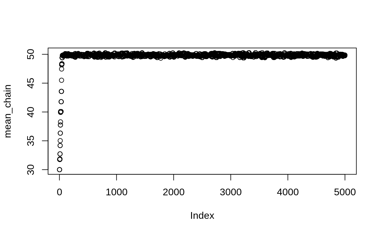
Figure 1: Trace plot of samples from one Metropolis algorithm

This shows the long road that our sampler takes to get from the starting value to the true mean. For this reason, typically we drop the beginning of the chain. These dropped samples are called the “burn in” period.

plot(mean_chain[100:n_samples], type = "l")

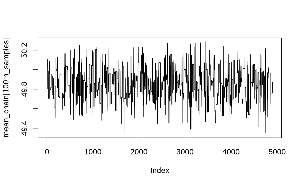
This shows the “fuzzy caterpillar” shape of a good, healthy Markov Chain.

hist(mean_chain[100:n_samples])
abline(v = M_true_mean, col = "green", lwd = 5)

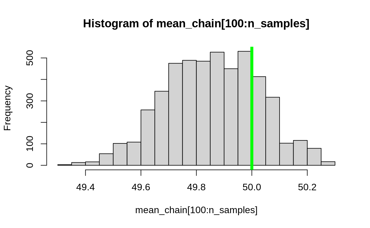
The green line shows the true average, which is close to the real value!

The weakness of Metropolis

Metropolis sampling will work, but sometimes we use MUCH more computer power than we need. Let’s see how many proposals are rejected in our sampling.

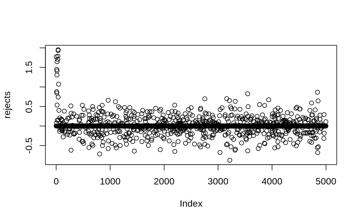
rejects <- zapsmall(mean_chain[2:n_samples] - mean_chain[1:(n_samples - 1)] )
# 
plot(rejects)

Figure 2: Rejection in the Metropolis algorithm. here values of 0 mean that the sampler kept the same value.

# 
n_rejects <- sum(rejects == 0)  / n_samples

We rejected 86.18% of the values we tried. That’s not very efficient! Soon we’ll see a more efficient way to do this.

Metropolis-Hastings Algorithm – asymmetrical jumps

See the slides on this part here

The same, but we can use an asymmetrical proposal distribution. This means that we can jump in either direction, but one direction is more likely. We need this, because sometimes our parameters are bounded! For example, the standard deviation of a normal distribution can never be negative.

Because our jumps are no longer symmetrical, we need to add a correction factor to our acceptance probability. Now, in addition to the Likelihood and Prior, we have the Candidate distribution getting involved:

\[ r = \frac{[y|\theta^{new}][\theta^{new}][\theta^{old}|\theta^{new}]} {[y|\theta^{old}][\theta^{old}][\theta^{old}|\theta^{new}]} \]

Here’s the same expression, but with more words substituted as a guide:

\[ r = \frac{\text{Likelihood}(\text{data}|\theta^{new}) \times \text{Prior}(\theta^{new}, \alpha, \beta) \times \text{Candidate}(\theta^{old}, \mu = \theta^{new}, \sigma_{tune})}{\text{Likelihood}(\text{data}|\theta^{old}) \times \text{Prior}(\theta^{old}, \alpha, \beta)\times \text{Candidate}(\theta^{new}, \mu = \theta^{old}, \sigma_{tune})} \]

once we have \(r\), we can get the probability of acceptance, \(R\), same as above (in the Metropolis algorithm):

\[ R = \text{min}( 1, r) \]

Let’s go (back) to our Normal weights example and try this out.

NOTE: We have to assume we KNOW the mean. Later we’ll see examples of what to do if you want to find two or more numbers at once!

Our model will be:

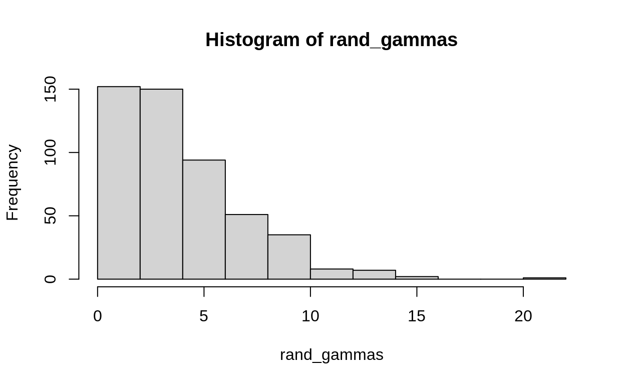
\[ \begin{align} y &\sim \text{Normal}(50, \sigma) \\ \sigma &\sim \text{Gamma}\left(\frac{4^2}{3^2}, \frac{4}{3^2}\right)\\ \end{align} \]

Why this weird notation for the gamma distribution?
Here I’m using a classic trick called moment matching. We do this because for almost all distributions with two parameters, the mean and standard deviation each depend on both parameters. This means that each parameter is also a function of both the mean and the standard deviation. That means we can’t directly set the mean and variance of a distribution with one parameter each.¹

Instead, we “reparameterize” the distribution, which just means we use values that correspond to the average and the standard deviation (or something like it). This is really helpful when you’re using these distributions for ecology!

for mean \(\mu\) and standard devation \(\sigma\), the Gamma distribution parameters are:

\[ \text{Gamma}\left(\frac{\mu^2}{\sigma^2}, \frac{\mu}{\sigma^2}\right) \]

here’s a quick demo to convince you:

rand_gammas <- rgamma(500, shape = 4^2/3^2, rate = 4/3^2)
hist(rand_gammas)

mean(rand_gammas) # close to 4

[1] 3.921929

sd(rand_gammas) # close to 3

[1] 2.949357

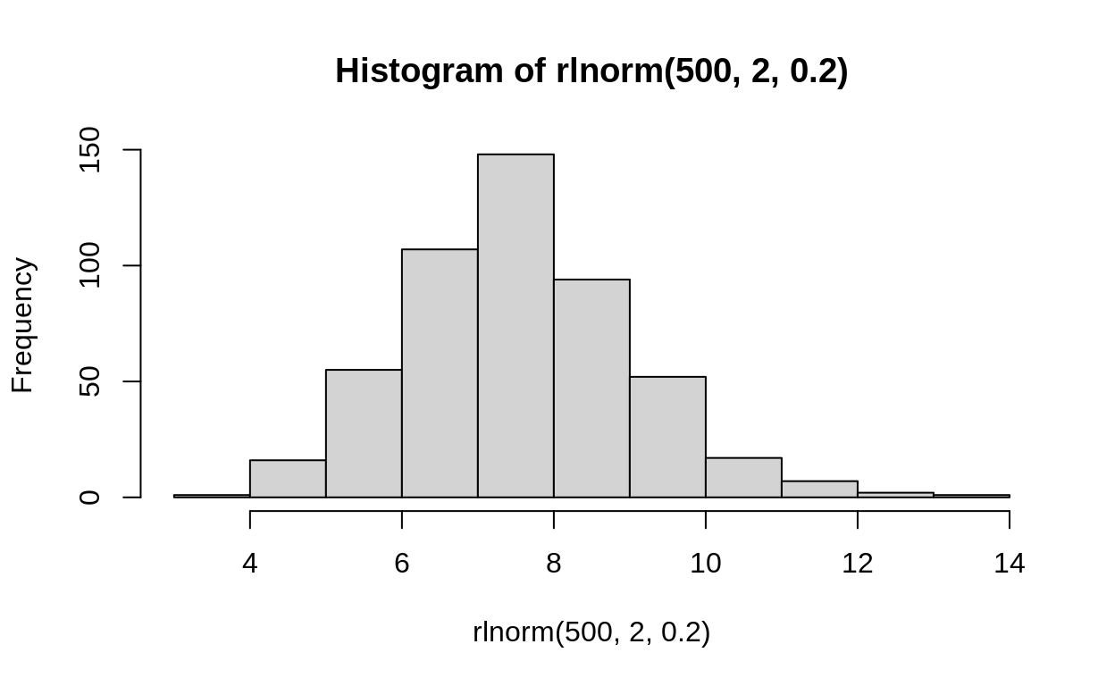
Proposal distribution

We also need a distribution for the proposals we will try in the algorithm. This distribution should be above 0, since we can’t have a 0 variance. The lognormal is a good choice (and is hopefully clear since it is not the same distribution as the gamma)

What does \(\text{lognormal}(2, 0.2)\) look like?

hist(rlnorm(500, 2, .2))

Code for Metropolis Hastings

Let’s do Metropolis Hastings. We begin as before, with an expression for the numerator of Bayes Rule:

## define likelihoods for our problem
MH_normal_loglike <- function(data_vec, sd_value){
  sum(dnorm(data_vec, mean = 50, sd = sd_value, log = TRUE))
}

######## ~~~!!!!!!!!!!!!!~~~~~~#########
## NOTE that the mean gets logged as it goes into rlnorm and dlnorm!! 
## This is a very necessary detail 
## read the help files (?rlnorm) to find out what the R functions expect
######## ~~~!!!!!!!!!!!!!~~~~~~#########

# proposal function to make new parameter values.
MH_propose_new_val <- function(old_value, sig_tune) {
  rlnorm(1, mean = log(old_value), sd = sig_tune)
}

MH_propose_density <- function(jump_to, jump_from, sig_tune) {
  dlnorm(x = jump_to, meanlog = log(jump_from), sdlog = sig_tune)
}


## function to use these to calculate the value of the numerator in Bayes Formula
## We are working on the LOG scale, so we have to ADD these together
MH_numerator <- function(v, data)  {
  # likelihood
  log_like <- MH_normal_loglike(data_vec = data, sd_value = v)
  # prior
  log_prior <- dgamma(x = v, shape = 4^2/3^2, rate = 4/3^2, log = TRUE)
  
  return(log_like + log_prior)
}

## function to calculate the acceptance ratio
MH_accept_probability <- function(new_value, old_value, 
                               data_to_use, 
                               tune_parameter) {
  
  # working on the LOG scale so we SUBTRACT values (the same as dividing these two things)
  new <- MH_numerator(v = new_value, data = data_to_use)
  old <- MH_numerator(v = old_value, data = data_to_use)
  
  difference_log_scale <- new - old
  
  # use EXP to undo the LOG
  r <- exp(difference_log_scale)
  
  # calculate the correction -- asymmetrical proposal
  new_from_old <- MH_propose_density(jump_to = new_value,
                                  jump_from = old_value,
                                  sig_tune = tune_parameter)
  
  old_from_new <- MH_propose_density(jump_to = old_value,
                                  jump_from = new_value,
                                  sig_tune = tune_parameter)
  
  R <- r * (old_from_new / new_from_old)
  
  p_accept <- min(1, R)
  
  return(p_accept)
}

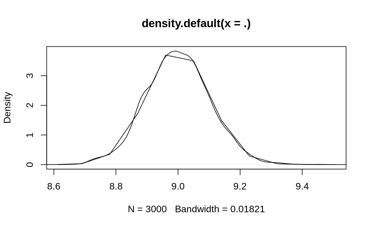
The proposal distribution, centered on a value (e.g. \(9\), to pick a random example) should be the same as the proposal density, centered on the same value.

replicate(3000, MH_propose_new_val(9, 0.1)) %>% hist(probability = TRUE)
curve(MH_propose_density(jump_to = x, jump_from = 9, sig_tune = 0.1), xlim = c(5,14), add = TRUE)

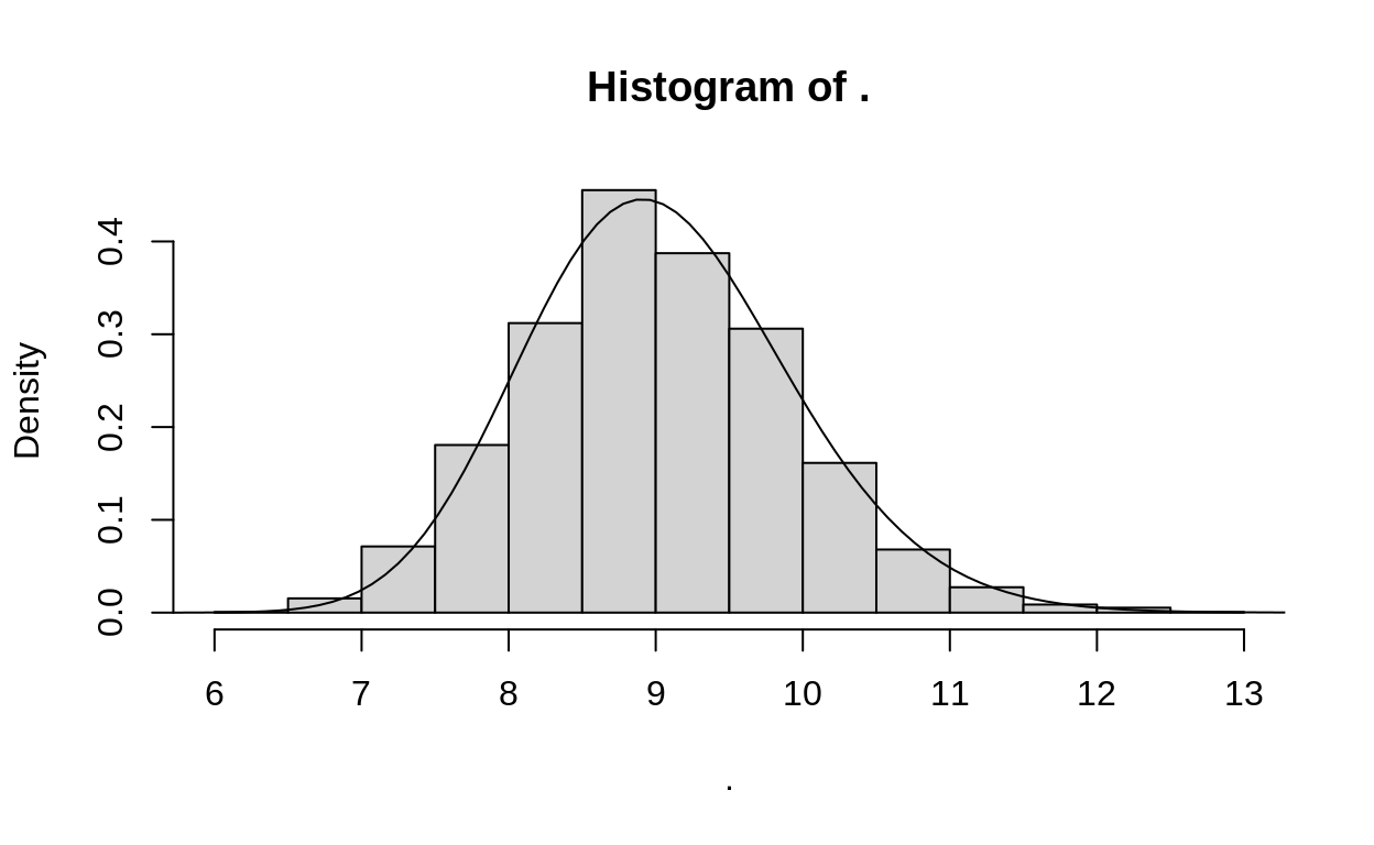
Quick comparison of random proposals, compared to the output of the proposal density function. This shows that the proposal density function is just giving us the probability of different values for the next proposal.

Figure 3: Quick comparison of random proposals, compared to the output of the proposal density function. This shows that the proposal density function is just giving us the probability of different values for the next proposal.

# set tune parameter
tune_parameter <- .2
# how long should the chain be? 
n_samples <- 5000

#start chain
sd_chain <- numeric(n_samples)

# start value
sd_chain[1] <- 7

for (i in 2:length(sd_chain)) {
  
  old_val <- sd_chain[i - 1]
  
  new_val <- MH_propose_new_val(old_value = old_val, sig_tune = tune_parameter)
  
  p_accept <- MH_accept_probability(new_value = new_val,
                                 old_value = old_val, 
                                 data_to_use = weights,
                                 tune_parameter = tune_parameter)
  
  sd_chain[i] <- ifelse(runif(1) < p_accept, new_val, old_val)
}



plot(sd_chain[300:n_samples], type = "l")
abline(h = correct_sd, col = "red")

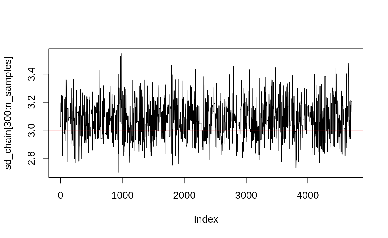
Figure 4: Metropolis Hastings chain for the posterior distribution of a standard deviation. Here we’ve dropped the burn-in period already.

plot(density(sd_chain[300:n_samples]))
abline(v = correct_sd)

median(sd_chain[300:n_samples])

[1] 3.072436

mean(sd_chain[300:n_samples])

[1] 3.074524

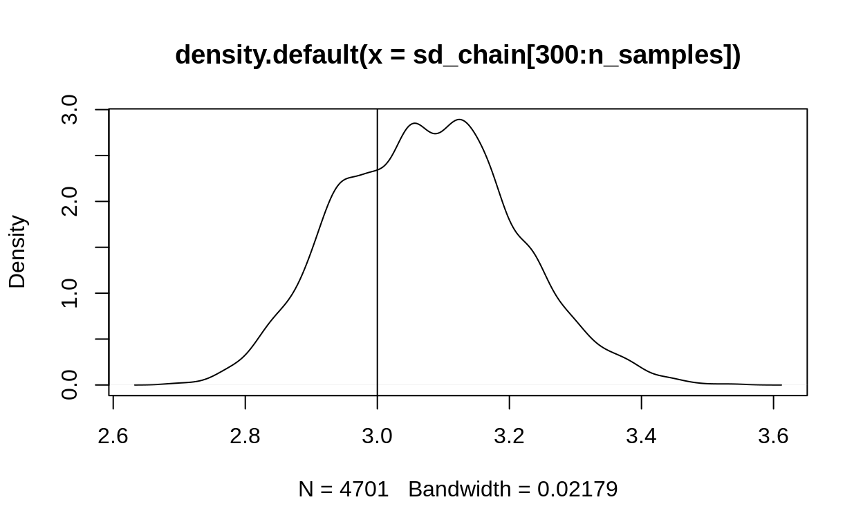
Close to the true value of correct_sd which is 3.

PSA: I made MANY errors while I was writing the above. If I had not started with simulated data, I would never have known!! Each time, I compared my answer to correct_sd and then went looking for the errors. Please remember to always do this, especially when you are coding an algorithm yourself!

Experiment with changing the proposal distribution! try for example gamma distribution:

MH_propose_new_val <- function(old_value, sig_tune) {
  rgamma(1, shape = old_value^2/sig_tune^2, rate = old_value/sig_tune^2)
}

MH_propose_density <- function(jump_to, jump_from, sig_tune) {
  dgamma(x = jump_to, shape = jump_from^2/sig_tune^2, rate = jump_from/sig_tune^2)
}

One Weird Trick to make calculating the posterior easy

Mean of a Normal Distribution

model is something like

\[ \begin{align} y &\sim \text{Normal}(\mu, 3) \\ \mu &\sim \text{Normal(40, 10)} \end{align} \]

if the variance is known, the posterior for the mean is a Normal distribution:

\[ \mu' \sim \text{Normal}\left(\frac{\frac{m}{s}+ \frac{\sum{y}}{\sigma^2}}{\frac{1}{s^2} + \frac{n}{\sigma^2}}, \left(\frac{1}{s^2} + \frac{n}{\sigma^2}\right)\right) \]

Note that \(m\) is the prior mean and \(s\) is the prior variance. This is the prior on the parameter \(\mu\), the mean of the distribution of the observations.

posterior_mean_calculate <- function(y_vector, known_sigma,
                      prior_mean, prior_sd,
                      n = length(y_vector)){
  numerator_mean <- (prior_mean/prior_sd^2 + sum(y_vector) / known_sigma^2)
  denominator_mean <- (1 / prior_sd^2 + n / known_sigma^2)
  
  new_mean <-  numerator_mean / denominator_mean
    
  new_var <- 1/denominator_mean
  
  return(list(mean = new_mean, sd = sqrt(new_var)))
}


## calculate the posterior distribution of the mean for the weights data
posterior_parameters <- posterior_mean_calculate(weights, 3, 
                                                 prior_mean = 30, 
                                                 prior_sd = 10)

hist(mean_chain[300:n_samples], probability = TRUE)
curve(dnorm(x, 
            mean = posterior_parameters$mean, 
            sd = posterior_parameters$sd), add = TRUE)

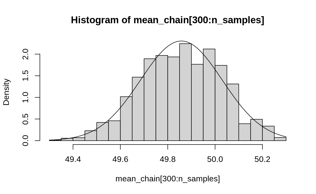
The Posterior distribution of the mean of a normal distribution. Here we find it two ways: first, using the conjugate prior. Second, using the Metropolis algorithm. You can see that the two are a close match.

Figure 5: The Posterior distribution of the mean of a normal distribution. Here we find it two ways: first, using the conjugate prior. Second, using the Metropolis algorithm. You can see that the two are a close match.

Variance of the Normal Distribution

First we need to do a little math tweak to the model:

\[ \begin{align} y &\sim \text{Normal}(50, \sigma) \\ \frac{1}{\sigma^2} &\sim \text{Gamma}\left(\frac{4^2}{3^2}, \frac{4}{3^2}\right)\\ \end{align} \]

Now instead of setting the prior on \(\sigma\) directly, we set the prior on the inverse square of sigma!²

We can think of this as a kind of link function. Doing a bit of algebra, we can see that:

\[ \begin{align} y &\sim \text{Normal}(50, g^{-1/2}) \\ g &\sim \text{Gamma}\left(\frac{4^2}{3^2}, \frac{4}{3^2}\right)\\ \end{align} \]

I admit that this makes setting reasonable priors awkward, so let’s go back to plotting:

gs <- rgamma(5000, 3.5^2/3^2, 3.5/3^2)

plot(density(gs^-.5))

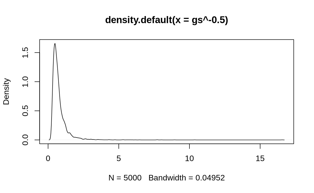
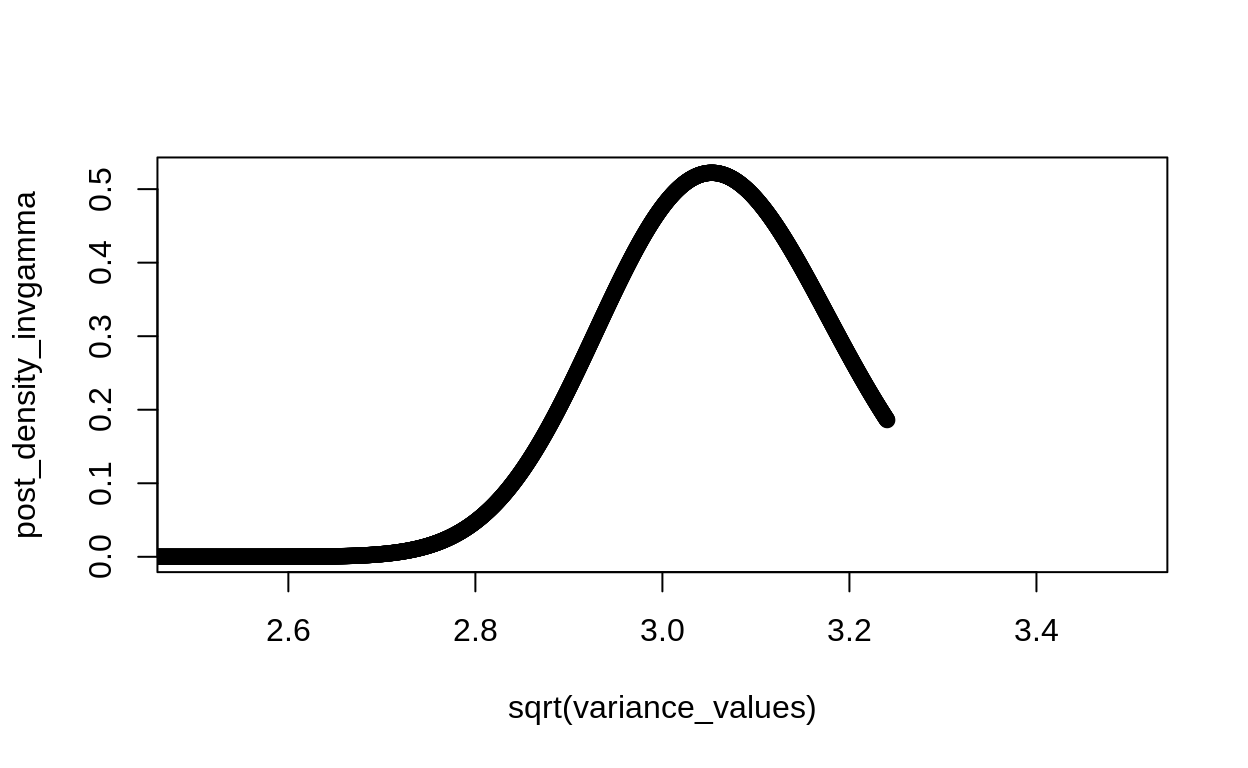
if the mean is known, then the posterior distribution for the variance is an inverse gamma:

\[ \frac{1}{\sigma^2} \sim \text{Gamma}\left(\alpha + \frac{n}{2}, \beta + \frac{\sum (y_i - \mu)^2}{2}\right) \]

Another, way less bothersome way to write this is with a related distribution, called the Inverse Gamma:

\[ \sigma^2 \sim \text{InvGamma}\left(\alpha + \frac{n}{2}, \beta + \frac{\sum (y_i - \mu)^2}{2}\right) \]

You can convert both precision and varience to the standard deviation with some algebra.

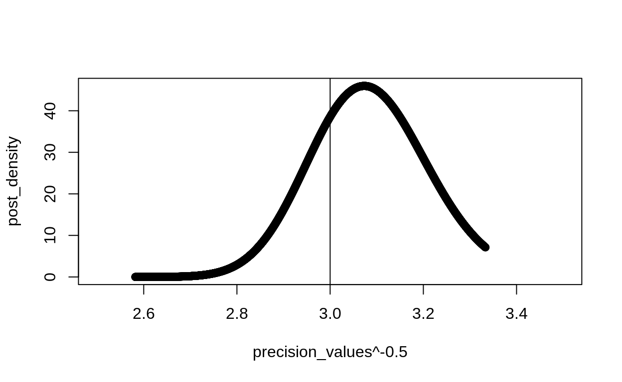
precision_values <- seq(0.09, .15, length.out = 3000)
post_density <- dgamma(precision_values, 2^2/50^2 + length(weights)/2, 2/5^2 + sum((weights - 50)^2)/2)

plot(x = precision_values^-.5, y = post_density, xlim = c(2.5,3.5))

(precision_values^-.5)[which.max(post_density)]

[1] 3.073139

abline(v = correct_sd)

equivalently:

variance_values <- seq(2.5, 10.5, length.out = 3000)
post_density_invgamma <- extraDistr::dinvgamma(variance_values,
                                alpha = 2^2/50^2 + length(weights)/2, 
                                beta = 2/5^2 + sum((weights - 50)^2)/2)

plot(x = sqrt(variance_values), y = post_density_invgamma, xlim = c(2.5,3.5))

posterior_sds <- tibble(sigma = seq(from = 2.6,
                                    to = 11,
                                    length.out = 500), 
                        density = extraDistr::dinvgamma(x = sigma,
                                                        alpha = 2^2/5^2 + length(weights)/2,
                                                        beta = (2/5^2 + sum((weights - 50)^2)/2)))

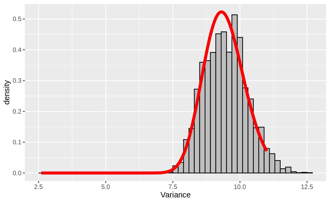
tibble(v = sd_chain[300:n_samples]) %>% 
  ggplot(aes(x = v^2)) +
  geom_histogram(aes(y = ..density..),
                 binwidth = .2, fill = "grey", color = "black") +
  geom_line(aes(x = sigma, y = density), 
            data = posterior_sds,
            col = "red", size = 2) + 
  labs(x = "Variance")

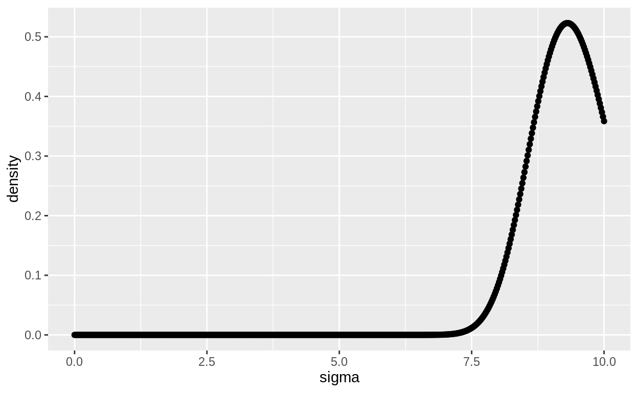
tibble(sigma = seq(from = 0, to = 10, length.out = 500), 
                          density = extraDistr::dinvgamma(x = sigma,
                                                          alpha = 2^2/5^2 + length(weights)/2,
                                                          beta = (2/5^2 + sum((weights - 50)^2)/2))) %>% 
  ggplot(aes(x = sigma, y = density)) + geom_point()

curve(extraDistr::dinvgamma(x = x,
                      alpha = 200,
                      beta = .1)
)

Gibbs sampling

Gibbs is like knitting

via GIPHY

Gibbs sampling is like knitting. Imagine you have several parameters and you’re going to take posterior samples for each one.

In this simple animation, each column is a parameter and each row is an iteration of the model.

Gibbs sampling works by simplifying a multivariate problem into small steps and tackling each one. We consider that all the parameters are known except the one we are sampling right now. Then, we sample form the posterior distribution for that parameter. This sampling can be done by conjugate posteriors, as we did above. It can also be done with the Metropolis or Metropolis-Hastings algorithm, or even with a combination of the two!

The steps for this algorithm are similar to the previous ones:

Start with random values for each parameter.
assuming that all are correct except the first, sample a value for the first.
Assuming that sample was correct for the first, sample the second.

Here is an example of the same thing in symbols, if that helps you to understand the process:

Consider a likelihood with two parameters, \(\alpha\) and \(\beta\). We have some observations, \(y\). We define prior distribution for \([\alpha]\) and \([\beta]\), \([\gamma]\) and we want to find the posterior distributions, conditional on the data :

\[ [\alpha, \beta , \gamma| y] \propto [y | \alpha, \beta, \gamma] [\alpha] [\beta] [\gamma] \]

Step 1 We assume that we know the true value of \(\alpha\) and \(\beta\), so the posterior depends only on \([\gamma]\) :

\[ [\gamma| y] \propto [y | \gamma] [\gamma] \]

We take a sample from this posterior

Step 2 We assume that we know the true value of \(\gamma\) and \(\beta\), so the posterior depends only on \([\alpha]\) :

\[ [\alpha| y] \propto [y | \alpha] [\alpha] \]

We take a sample from this posterior

Step 1 We assume that we know the true value of \(\gamma\) and \(\alpha\), so the posterior depends only on \([\beta]\) :

\[ [\beta| y] \propto [y | \beta] [\beta] \]

We take a sample from this posterior.

Do this “lots” (many thousands) of times and, if all goes well, you get something that approaches the full posterior distribution.

How do we draw these samples? There are many ways, and we have just seen three of the favourite classics: Metropolis, Metropolis-Hastings, and Conjugate Priors.

In Gibbs sampling, we draw samples by assuming that we know all the parameters except the first. Then we assume we know all except the second, then all except the third. This is very similar to above, where we used conjugate priors for calculating the posterior of the mean (using the true variance), and then again the posterior for the variance (using the true mean). In the examples above (in the “One Weird Trick” section) we made use of the correct values for the parameter we assumed we knew. In Gibbs sampling you don’t know – so you start with a random guess instead. As you iterate back and forth across the parameters, your guesses improve and improve until, wondrously, you end up sampling the full and correct posterior.

Gibbs is like swimming

Swimming Freestyle Swimming GIFfrom Swimming GIFs

Gibbs sampling is also like freestyle swimming. From Wikipedia :

The term ‘freestyle stroke’ is sometimes used as a synonym for ‘front crawl’,[3] as front crawl is the fastest swimming stroke. It is now the most common stroke used in freestyle competitions.

While technically swimmers could use any stroke in Freestyle events, they overwhelmingly prefer the Front Crawl because it is the fastest. So much so that many people call the Front Crawl stroke itself the “Freestyle”.

Gibbs sampling is like this. While, technically, you can use any algorithm you like to sample from the univariate distributions described above – people use one far more than the others. The use of Conjugate Priors is so incredibly fast compared to all other ways of getting the posterior that Gibbs sampling is nearly synonymous with it. All we have to do is deliberately choose our priors to be conjugates, and we can save huge amounts of time and effort.³

Gibbs demonstration with the Normal Distribution

Let’s begin by simulating some values from a normal distribution:

true_mean <- 31
true_sd <-  4
sample_size <- 30
set.seed(1859)
mass_values <- rnorm(n = sample_size, mean = true_mean, sd = true_sd)

hist(mass_values)

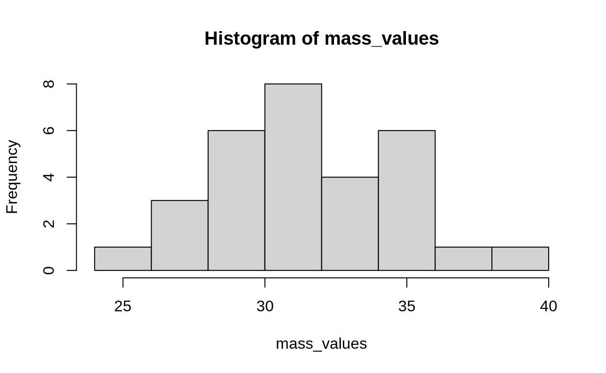
We define a model for these data. We do this in a very deliberate way, choosing the priors to be conjugates:

\[ \begin{align} y &\sim \text{Normal}(\mu, \sigma) \\ \mu &\sim \text{Normal}(10,5) \\ \frac{1}{\sigma^2} &\sim \text{Gamma}(4.1^2/2^2, 4.1/2^2) \end{align} \]

Why did I choose the mean of 4.5 for the gamma distribution? What is a gamma distribution anyway, and what does this strange link function mean?

As usual, simulation is a great way to understand and practice.

Let’s start by simulating values with a mean of 4.1 and a standard devation of 2 from a gamma distribution:

sample_precision <- rgamma(1000, shape = 4.1^2/2^2, rate = 4.1/2^2)
mean(sample_precision)

[1] 4.019667

sd(sample_precision)

[1] 1.903422

curve(dgamma(x, shape = 3^2/2^2, rate = 3/2^2), xlim = c(0, 5))

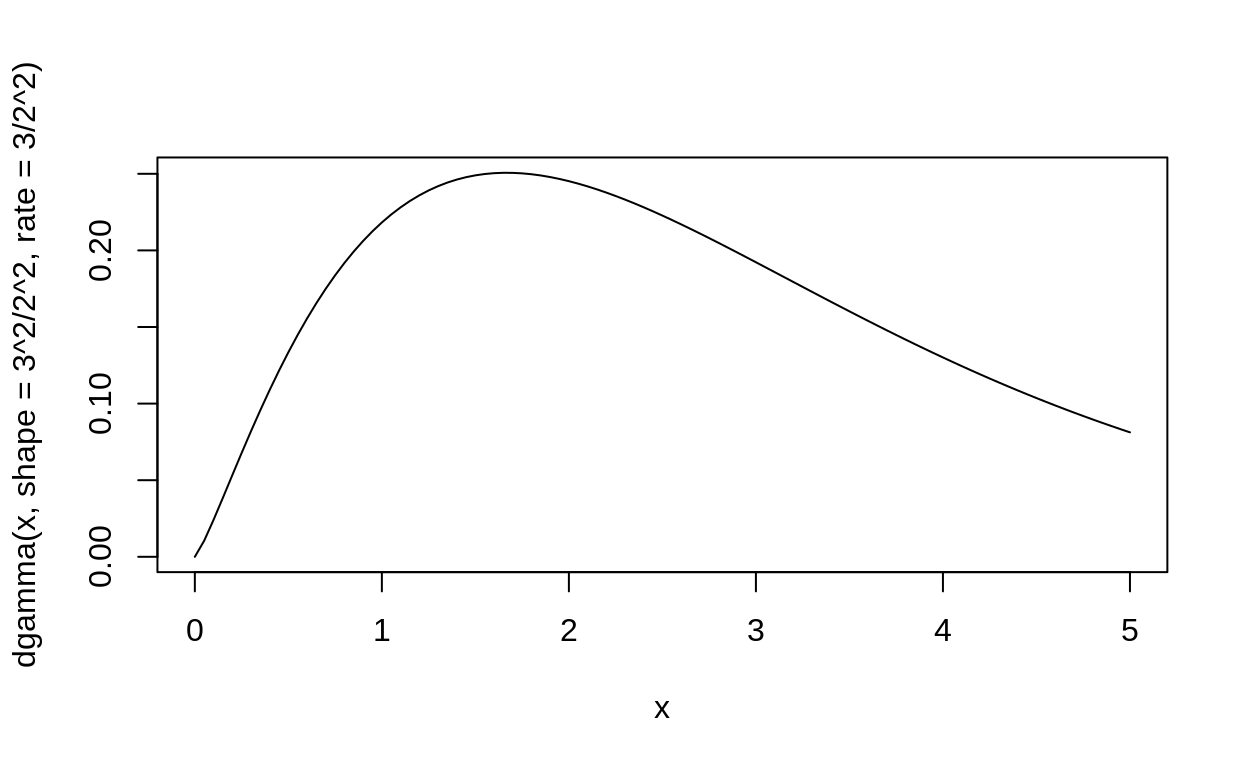
These values are what are called “precision”, and they are a favourite way to think about the Normal distribution. Precision is the inverse of the variance, so it has the opposite effect: When variance is large, the Normal distribution is flatter. When the precision is large, the distribution is narrower and concentrated close to the mean.

If \(1/\sigma^2\) is the precision (often written \(\tau\)) then:

\[ \sigma = \frac{1}{\sqrt \tau} \]

And we can calculate this:

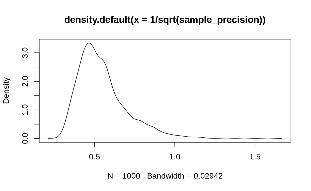
plot(density(1/sqrt(sample_precision)))

Figure 6: This shows the standard deviations implied by the gamma distribution above.

Defining and running a Gibbs Sampler

To implement this model we need to write functions that will do each of these things in turn.

First we set up two functions that simply compute the equations above for the conjugate posteriors. Once we have that distribution, we draw a random sample from it and the function returns that value.

# calculate the posterior normal distribution for the data and a known variance

post_mean <- function(y_vector, known_sigma,
                      prior_mean, prior_sd,
                      n = length(y_vector)){
  numerator_mean <- (prior_mean/prior_sd^2 + sum(y_vector) / known_sigma^2)
  denominator_mean <- (1 / prior_sd^2 + n / known_sigma^2)
  
  new_mean <-  numerator_mean / denominator_mean
    
  new_var <- 1/denominator_mean
  
  rnorm(1, mean = new_mean, sd = sqrt(new_var))
}

# fun to play with this! make sure it makes sense! 
post_mean(y_vector = c(2,4,1,5), .1, 7, 2)

[1] 2.984141

We implement the equation for the posterior of \(\sigma\) in the same way.

post_sd <- function(y_vector, known_mean, prior_alpha, prior_beta){
  
  new_alpha <- prior_alpha + length(y_vector) / 2
  
  new_beta <- prior_beta + sum((y_vector - known_mean)^2) / 2
  
  inverse_variance <- rgamma(n = 1, shape = new_alpha, rate = new_beta)
  
  sd_sample <- sqrt(1/inverse_variance)
  return(sd_sample)
}

post_sd(c(2,4,1,5), known_mean = 3, prior_alpha = 2^2/2^2, prior_beta = 2/2^2)

[1] 1.126258

Running the sampler means alternating between these two functions. In each iteration, we take the results of the previous sample and feed them into the next sample.

true_mean <- 24
true_sd <- 7

y_data <- rnorm(400, mean = true_mean, sd = true_sd)

# gibbs process
n_iterations <- 2000
mean_chain <- numeric(n_iterations)
sd_chain <- numeric(n_iterations)


# sample to start -- could be anything, might as well be priors
mean_chain[1] <- rnorm(1, mean = 10, sd = 5)
sd_chain[1] <- rgamma(1, shape = 3^2/2^2, rate = 3/2^2)

for (k in 2:n_iterations) {
  # draw a mean
  mean_chain[k] <- post_mean(y_vector = y_data,
                             known_sigma = sd_chain[k - 1],
                             prior_mean = 10,
                             prior_sd = 5)
  sd_chain[k] <- post_sd(y_vector = y_data, 
                         known_mean = mean_chain[k],
                         prior_alpha = 3^2/2^2,
                         prior_beta = 3/2^2)
}

par(mfrow = c(1,2))
plot(mean_chain, type = "l")
abline(h = true_mean, col = "red", lwd = 2)
plot(sd_chain, type = "l")
abline(h = true_sd, col = "red", lwd = 2)

par(mfrow = c(1,1))

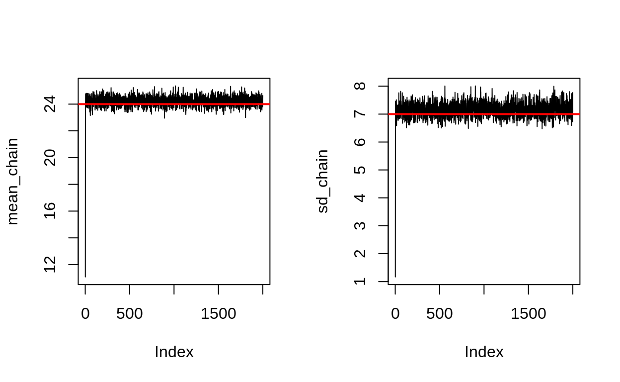
You can see that the chains are almost exactly what we want.

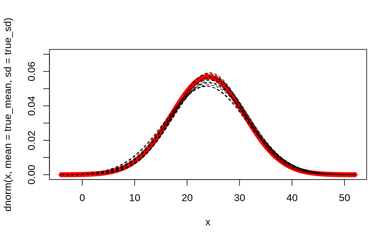
Another way to check our result is to draw a few of the normal curves that our data suggests.

curve(dnorm(x, mean = true_mean, sd = true_sd),
      xlim = c(true_mean - 4 * true_sd,
               true_mean + 4 * true_sd), 
      lwd = 8, col = "red", ylim = c(0, 0.07))

for (i in (n_iterations-10):n_iterations) {
  curve(dnorm(x, mean = mean_chain[i], sd = sd_chain[i]), add = TRUE, lty = 2)
}

Are the posterior medians close to the real values?

median(mean_chain[100:n_iterations])

[1] 24.22588

true_mean

[1] 24

median(sd_chain[100:n_iterations])

[1] 7.153504

true_sd

[1] 7

We can also look at the pairs plot, like this

plot(mean_chain[100:n_iterations], sd_chain[100:n_iterations])

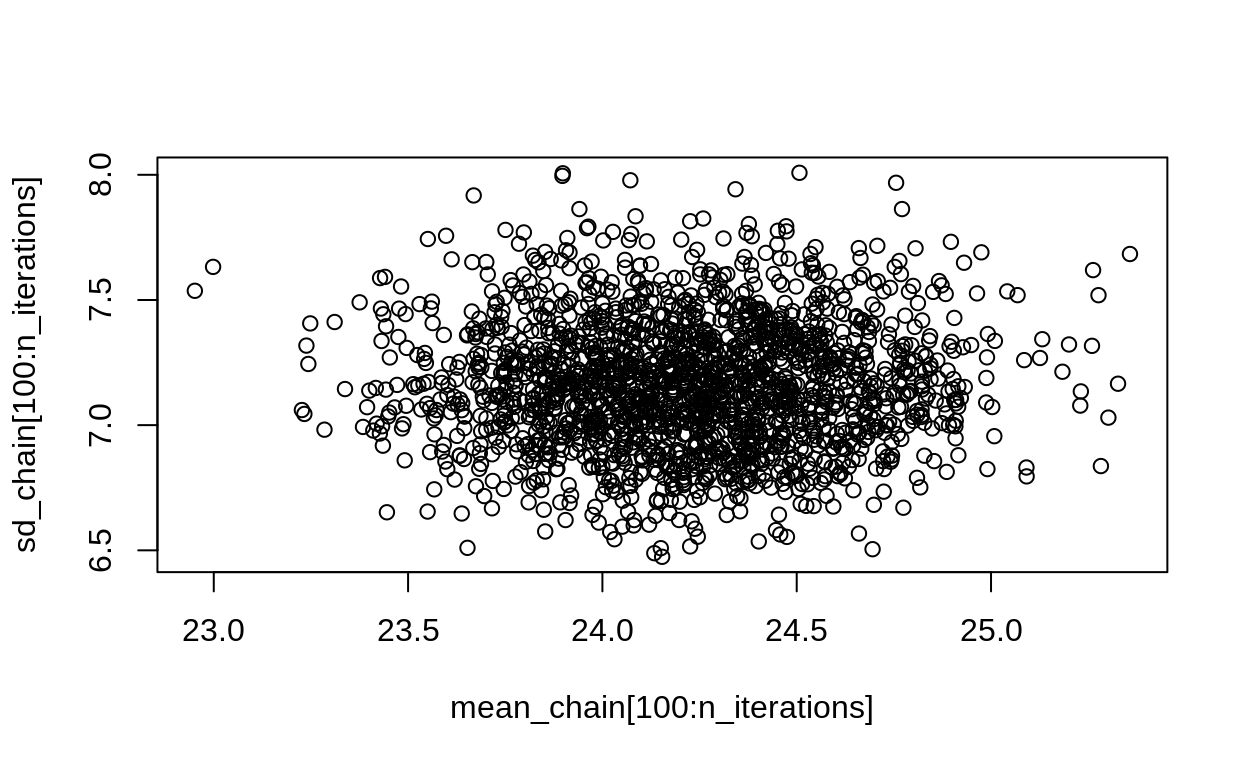
This reveals if there are any correlations in the posterior.

Metropolis-in-Gibbs

Sometimes we need a Deluxe option – running a Metropolis Hastings sampler inside a Gibbs sampler

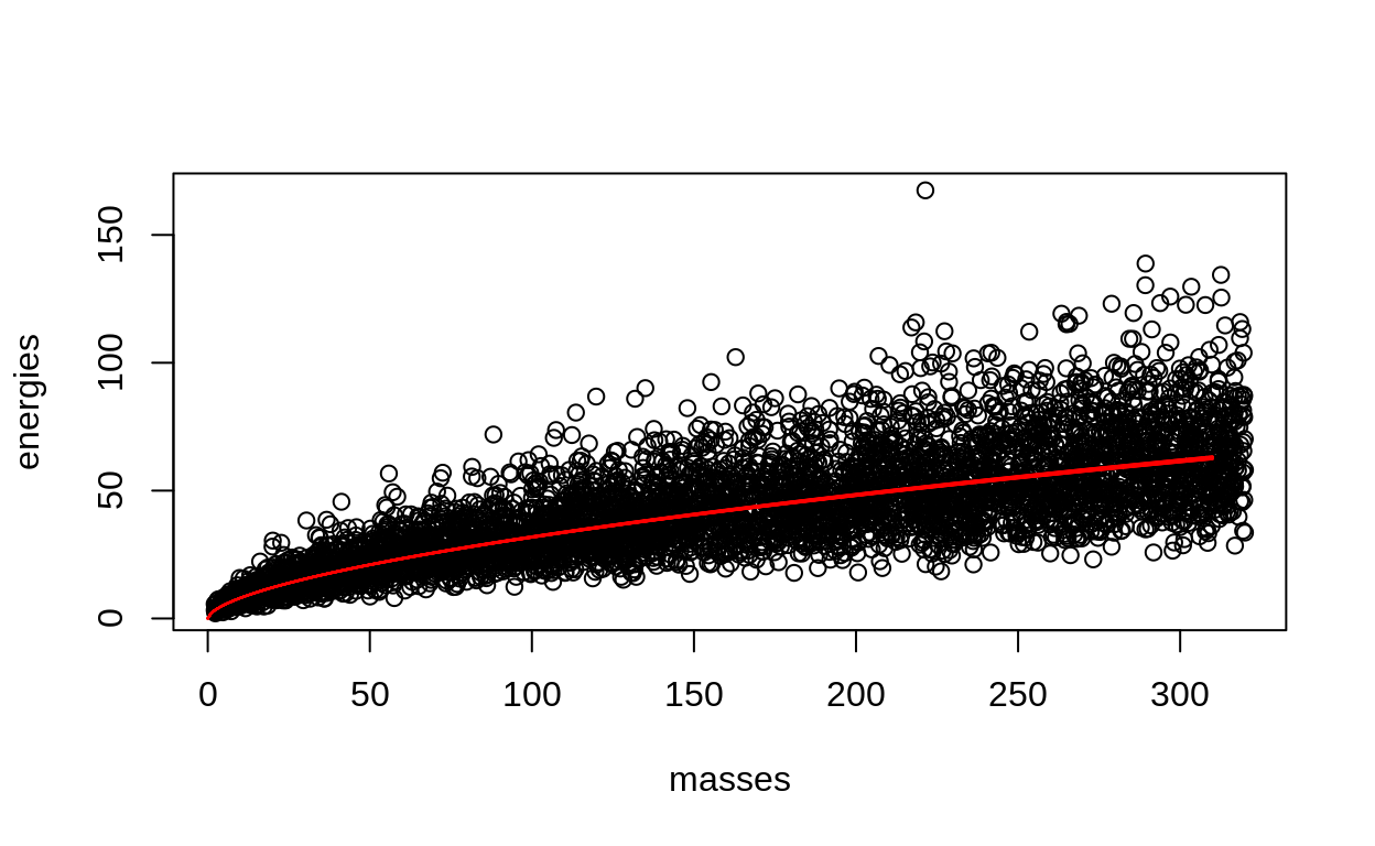
Let’s look at an example where that is necessary: metabolism and body size.⁴

\[ \begin{align} \text{Metabolism} &\sim \text{LogNormal}(\text{log}(\alpha), \beta) \\ \alpha &= c \times \text{Mass}^d \\ c &\sim \text{gamma}\left(\frac{3^2}{2^2}, \frac{3}{2^2}\right) \\ \text{logit}(d) &\sim \text{Normal}(0, 0.5) \\ \beta &\sim \text{InvGamma(3, 4)} \end{align} \]

Some notes on this model:

Metabolism can’t be negative, so we model it with a distribution that also can’t be negative – in this case, the LogNormal distribution.
The LogNormal has two parameters. Here I’m calling the \(\alpha\) and \(\beta\). Sometimes people call them \(\mu\) and \(\sigma\), but I find that confusing because they are not the mean and the standard deviation. For now, just know that \(\alpha\) is the median of the data and \(\beta\) is the “spread” around it.
\(\alpha\) is not a parameter in our model, but just a placeholder for our deterministic function, \(c \times \text{Mass}^d\).
Since the response can’t be negative, and body mass can’t be negative, that means the constant \(c\) can’t be negative either! So here we guarantee it by using a bounded prior.
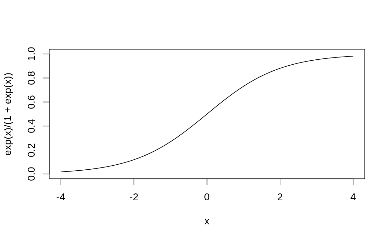
Metabolic relationships are always decelerating curves – this means that the exponent is always between 0 and 1. Here we guarantee that it will be there by using a logit link function. This means that we can use a symmetrical prior like the Normal distribution.⁵

Let’s simulate from this model! This will let us see how it works. We’ll then use the data to write a Metropolis-In-Gibbs approach that uses all three of the techniques we’ve seen

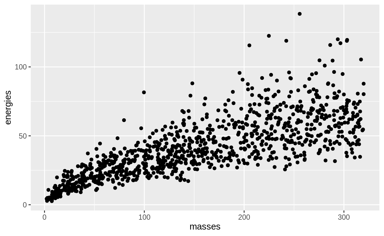
Simulating metabolic data

Our first step is to simulate from the model above! The workflow goes like this:

Set true values for \(c\), \(d\) and \(\beta\). Later we’ll use these to verify if we have the correct information.
Create a fake vector of Mass values. We imagine they are evenly spaced over a reasonable range.
Calculate the median Metabolic rate (a.k.a “Energy”, our response).
Simulate observations around that median value.

This code does these steps:

true_beta <- .3
true_constant <-  2
true_exponent <- .6
sample_size <- 5000
set.seed(1859)

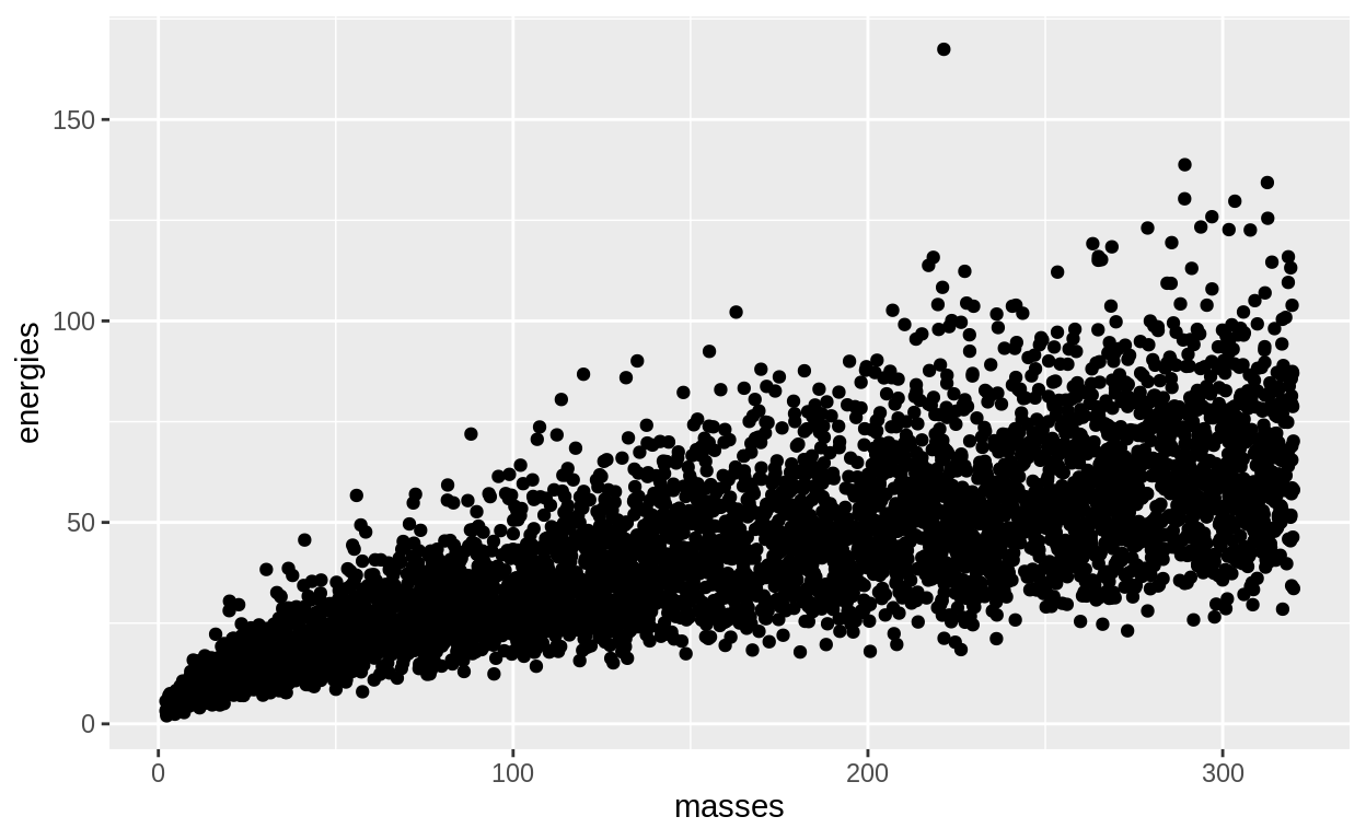
energy_mass <- tibble(
  masses = runif(n = sample_size, min = 2, max = 320),
  med_energy = true_constant*masses^true_exponent,
  energies = rlnorm(n = sample_size,
                    meanlog = log(med_energy), 
                    sdlog = true_beta))

data_figure <- energy_mass %>% 
  ggplot(aes(x = masses, y = energies)) + geom_point()
data_figure

Setting up the three sampling approaches

Mean and likelihood

We need a function to calculate the deterministic part of the model. Note that this is a good place to add any link functions that we’re using.

calculate_alpha <- function(constant, logit_exponent, mass_data){
  
  inv_logit <- function(x) exp(x)/(1 + exp(x))
  
  exponent_zero_one <- inv_logit(logit_exponent)
  
  median_energy <- constant * mass_data ^ exponent_zero_one
  
  return(median_energy)
}

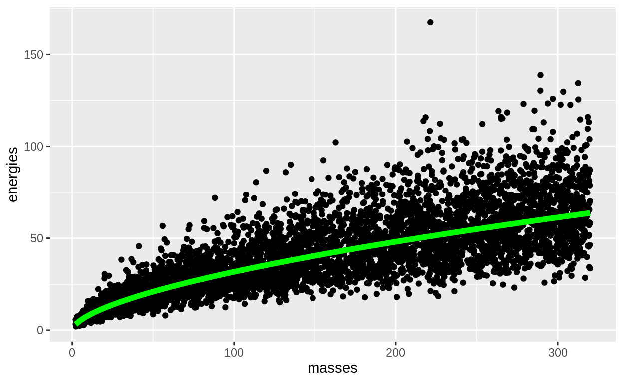
data_figure + 
  stat_function(fun = function(x) calculate_alpha(
                        constant = true_constant,
                        logit_exponent = qlogis(true_exponent),
                        mass_data = x), lwd = 2, col = "green")

We also need a handy function to take the three parameters (constant, logit_exponent and beta) and use them to calculate the likelihood of the data:

loglike_energy <- function(constant, logit_exponent, beta, mass_data, energy_data){
  
  alpha <- calculate_alpha(constant = constant,
                           logit_exponent = logit_exponent,
                           mass_data = mass_data)
  
  log_like_datapoints <- dlnorm(x = energy_data, 
                                meanlog = log(alpha), 
                                sdlog = beta, 
                                log = TRUE)
  
  return(sum(log_like_datapoints))
}

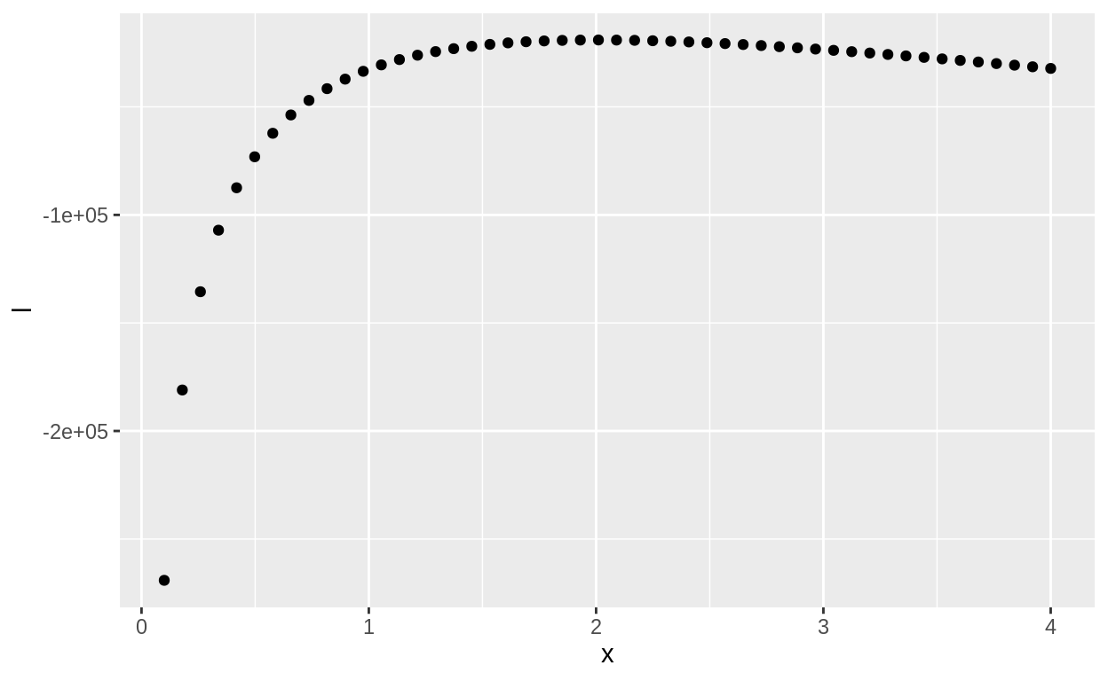
tibble(x = seq(.1, 4, length.out = 50),
       l = map_dbl(x, ~ loglike_energy(logit_exponent = qlogis(true_exponent),
                           constant = .x, 
                           beta = true_beta,
                           energy_data = energy_mass$energies,
                           mass_data = energy_mass$masses))) %>% 
  ggplot(aes(x = x, y = l)) + geom_point()

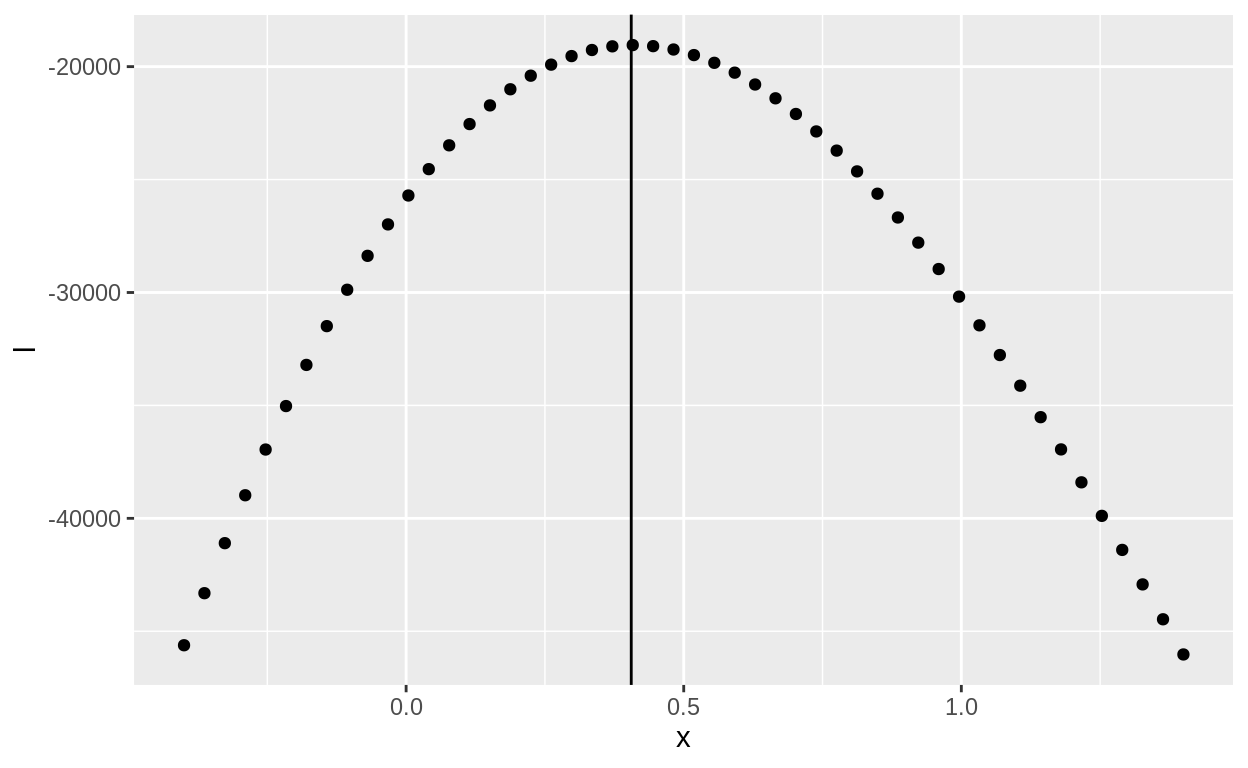
tibble(x = seq(-.4, 1.4, length.out = 50),
       l = map_dbl(x, ~ loglike_energy(logit_exponent = .x,
                           constant = true_constant, 
                           beta = true_beta,
                           energy_data = energy_mass$energies,
                           mass_data = energy_mass$masses))) %>% 
  ggplot(aes(x = x, y = l)) + 
  geom_point() + 
  geom_vline(xintercept = qlogis(true_exponent))

\(\beta\): Conjugacy and the lognormal

If we assume we know \(\text{log}(\alpha)\) (i.e. the true median) then the distribution of the data depends only on \(\beta\). This parameter represents the standard deviation of the log of the LogNormal distribution. That is, if you log-transform a LogNormal distribution you get a Normal distribution. This is the standard deviation of that distribution.

Not surprisingly, the Conjugate Posterior looks very similar:

\[ \begin{align} [\beta | y] &\propto \text{LogNormal}(y | \beta) \times \text{InvGamma}(3,4) \\ &= \text{InvGamma}\left(3 + \frac{n}{2}, 4 + \frac{\sum\big(\text{log}(y) - \text{log}(\alpha)\big)^2 }{ 2}\right) \end{align} \]

For an exploration of this, take a look at the Appendix “exploring the Inverse Gamma”.

So we simply need a function that takes the “known” value of \(\alpha\) and returns a sample from the posterior for \(\beta\)

sample_beta <- function(y, alpha){
  one_variance <- extraDistr::rinvgamma(1, 
                        alpha = 50 + length(y)/2,
                        beta = 4 + sum( (log(y) - log(alpha))^2 ) / 2)
  
  one_sd <- sqrt(one_variance)
  
  return(one_sd)
}

\(b\): the Metropolis algorithm

Because \(b\) is modeled on the logit scale, we can use a symmetrical prior and a symmetrical proposal distribution. This means we don’t need the Metropolis-Hastings correction for asymmetrical proposals.

Here we assume that \(c\) (constant) and \(\beta\) (beta) are known.

# proposal function to make new parameter values.
Metropolis_propose_new_val <- function(old_value, tune) {
  runif(1, min = old_value - tune, max = old_value + tune)
}

# we also need a function for the prior
calculate_exponent_prior_logprob <- function(x){
  dnorm(x = x, mean = 0, sd = 0.5, log = TRUE)
}

quick demo

log_like <- loglike_energy(logit_exponent = .4,
                           constant = true_constant, 
                           beta = true_beta,
                           energy_data = energy_mass$energies,
                           mass_data = energy_mass$masses)
# prior
log_prior <- calculate_exponent_prior_logprob(.4)


## We are working on the LOG scale, so we have to ADD these together
# This gives us the NUMERATOR of Bayes formula: the likelihood X the prior
log_like + log_prior

[1] -19048.84

We need a function to calculate the metropolis acceptance probability. Note that I’ve changed this from above – instead of calculating the numerator INSIDE this function, now I’m assuming we already calculated the values for the new (proposal) numerator and the old (previous iteration) numerator. As a reminder, the “numerator” refers to the numerator of Bayes formula: the likelihood of the data multiplied by the prior.

## function to calculate the acceptance probability
Metropolis_accept_probability <- function(new_numerator_log, 
                                          old_numerator_log) {
  
  # working on the LOG scale so we SUBTRACT values (the same as dividing these two things)
  difference_log_scale <- new_numerator_log - old_numerator_log
  
  # use EXP to undo the LOG -- convert back to probability
  r <- exp(difference_log_scale)
  
  p_accept <- min(1, r)
  
  return(p_accept)
}

# the "correct" value is log(true_exponent/(1-true_exponent)), so around .405
# we can play around that value to see acceptance probabilities less than 1
Metropolis_accept_probability(
  new_numerator_log = 
    loglike_energy(logit_exponent = .399,
                   constant = true_constant, 
                   beta = true_beta,
                   energy_data = energy_mass$energies,
                   mass_data = energy_mass$masses) + 
    calculate_exponent_prior_logprob(.399),
  old_numerator_log = 
    loglike_energy(logit_exponent = .4,
                   constant = true_constant, 
                   beta = true_beta,
                   energy_data = energy_mass$energies,
                   mass_data = energy_mass$masses) + 
    calculate_exponent_prior_logprob(.4))

[1] 0.4617771

Put it all together:

sample_exponent_Metropolis <- function(exponent_previous_val,
                              constant_known,
                              beta_known,
                              energy_dat = energy_mass$energies,
                              mass_dat = energy_mass$masses,
                              metropolis_tune){
  # 
  
  prev_log_prior_exponent<- calculate_exponent_prior_logprob(exponent_previous_val)
  
  prev_log_like_data <- loglike_energy(logit_exponent = exponent_previous_val,
                   constant = constant_known, 
                   beta = beta_known,
                   energy_data = energy_dat,
                   mass_data = mass_dat)
  
  ## propose new!
  exponent_propose_val <- Metropolis_propose_new_val(old_value = exponent_previous_val,
                                                     tune = metropolis_tune)
  

  propose_log_prior_exponent<- calculate_exponent_prior_logprob(exponent_propose_val)
  
  propose_log_like_data <- loglike_energy(logit_exponent = exponent_propose_val,
                   constant = constant_known, 
                   beta = beta_known,
                   energy_data = energy_dat,
                   mass_data = mass_dat)

  p_accept <- Metropolis_accept_probability(
    new_numerator_log = propose_log_prior_exponent + propose_log_like_data,
    old_numerator_log = prev_log_prior_exponent + prev_log_like_data)
  
  next_val <- ifelse(runif(1) < p_accept,
                     yes = exponent_propose_val, 
                     no = exponent_previous_val)
  
  return(next_val)
}

\(c\): the Metropolis-Hastings algorithm

This is going to be the same as above, with one addition. Here we need to use an asymmetrical proposal distribution and also add a correction for it! I’ve copied this code down from the “Code for Metropolis” section above. Reread that section for more details!

# proposal function to make new parameter values.

######## ~~~!!!!!!!!!!!!!~~~~~~#########
## NOTE that the mean gets logged as it goes into rlnorm and dlnorm!! 
## This is a very necessary detail 
## read the help files (?rlnorm) to find out what the R functions expect
######## ~~~!!!!!!!!!!!!!~~~~~~#########

# proposal function to make new parameter values.
MH_propose_new_val <- function(old_value, sig_tune) {
  # rlnorm(1, mean = log(old_value), sd = sig_tune)
  rgamma(1, shape = old_value^2/sig_tune^2, rate = old_value/sig_tune^2)
}

MH_propose_density <- function(jump_to, jump_from, sig_tune) {
  # dlnorm(x = jump_to, meanlog = log(jump_from), sdlog = sig_tune)
  dgamma(jump_to, shape = jump_from^2/sig_tune^2, rate = jump_from/sig_tune^2)
}


# calculate the correction factor
calculate_correction <- function(new_value, old_value, tune_parameter){
  # calculate the correction -- asymmetrical proposal
  new_from_old <- MH_propose_density(jump_to = new_value,
                                     jump_from = old_value,
                                     sig_tune = tune_parameter)
  
  old_from_new <- MH_propose_density(jump_to = old_value,
                                     jump_from = new_value,
                                     sig_tune = tune_parameter)
  
  return(old_from_new / new_from_old)
}

MetropolisHastings_accept_probability <- function(new_numerator_log, 
                                                  old_numerator_log, 
                                                  correction) {
  
  # working on the LOG scale so we SUBTRACT values (the same as dividing these two things)
  difference_log_scale <- new_numerator_log - old_numerator_log
  
  # use EXP to undo the LOG -- convert back to probability
  r <- exp(difference_log_scale)
  
  R <- r * correction
  
  p_accept <- min(1, R)
  
  return(p_accept)
}

Check these, same as above:

replicate(3000, MH_propose_new_val(9, 0.1)) %>% density %>% plot
curve(MH_propose_density(jump_to = x, jump_from = 9, sig_tune = 0.1), xlim = c(5,14), add = TRUE)

Again, I’ve made a minor change to the code. Here I’ve taking the calculation of the “correction factor” and pulled it out into its own function. Hopefully this makes the workflow clearer!

our prior for c was

\[ c \sim \text{gamma}\left(\frac{3^2}{2^2}, \frac{3}{2^2}\right) \]

Let’s wrap up all the steps of the Metropolis Hastings process into one function:

# we also need a function for the prior
calculate_constant_prior_logprob <- function(x){
  dgamma(x = x, shape = 3^2/2^2, rate = 3/2^2, log = TRUE)
}

sample_constant_MetropolisH <- function(constant_previous_val,
                               exponent_known,
                               beta_known,
                               energy_dat = energy_mass$energies,
                               mass_dat = energy_mass$masses,
                               MH_tune){
  # 
  
  prev_log_prior_constant <- calculate_constant_prior_logprob(constant_previous_val)
  
  prev_log_like_data <- loglike_energy(
    logit_exponent = exponent_known,
    # the next line is for the parameter we are sampling! 
    constant = constant_previous_val, 
    beta = beta_known,
    energy_data = energy_dat,
    mass_data = mass_dat)
  
  ## propose new!
  constant_propose_val <- MH_propose_new_val(constant_previous_val,
                                             sig_tune = MH_tune)
  

  propose_log_prior_constant <- calculate_constant_prior_logprob(constant_propose_val)
  
  propose_log_like_data <- loglike_energy(
    logit_exponent = exponent_known,
    # next line is for the parameter we are trying next!
    constant = constant_propose_val, 
    beta = beta_known,
    energy_data = energy_dat,
    mass_data = mass_dat)
  
  ## Correction! the special step of MH
  correction <- calculate_correction(new_value = constant_previous_val,
                                     old_value = constant_propose_val,
                                     tune_parameter = MH_tune)
  

  p_accept <- MetropolisHastings_accept_probability(
    new_numerator_log = propose_log_prior_constant + propose_log_like_data,
    old_numerator_log = prev_log_prior_constant + prev_log_like_data,
    correction = correction)
  
  next_val <- ifelse(runif(1) < p_accept,
                     yes = constant_propose_val, 
                     no = constant_previous_val)
  
  return(next_val)
}

Combine all three

n_iter <- 15000
gibbs_chain <- list(constant = numeric(n_iter),
                    exponent = numeric(n_iter),
                    beta     = numeric(n_iter))


# start value
gibbs_chain$constant[1] <- 2.5
gibbs_chain$exponent[1] <- .5
gibbs_chain$beta[1] <- .1


for (k in 2:n_iter) {
        
  # constant
  gibbs_chain$constant[k] <- sample_constant_MetropolisH(
    constant_previous_val = gibbs_chain$constant[k - 1],
    exponent_known = gibbs_chain$exponent[k - 1],
    beta_known = gibbs_chain$beta[k - 1],
    MH_tune = .1)
  
  #exponent
  gibbs_chain$exponent[k] <-  sample_exponent_Metropolis(
    exponent_previous_val = gibbs_chain$exponent[k-1],
    constant_known = gibbs_chain$constant[k],
    beta_known = gibbs_chain$beta[k - 1],
    metropolis_tune = .2)
  
  #beta
  gibbs_chain$beta[k] <- sample_beta(y = energy_mass$energies,
                                     alpha = calculate_alpha(
                                       constant = gibbs_chain$constant[k],
                                       logit_exponent = gibbs_chain$exponent[k],
                                       mass_data = energy_mass$masses
                                     ))
}

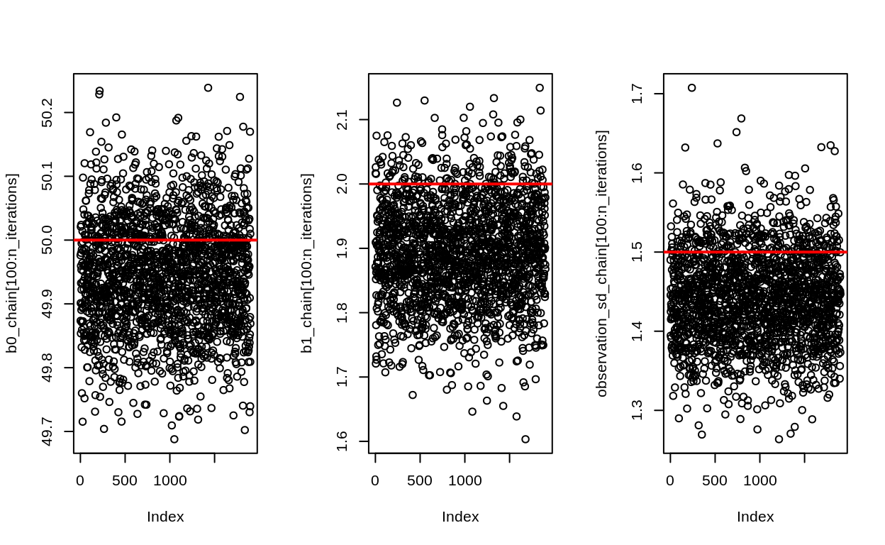
real_param <- tribble(~parameter, ~truth,
        "beta", true_beta,
        "constant", true_constant,
        "exponent", qlogis(true_exponent))

gibbs_chain %>% as_tibble() %>% 
  mutate(iter = 1:n_iter) %>% 
  filter(iter > 300) %>% 
  pivot_longer(-iter, names_to = "parameter", values_to = "value") %>% 
  ggplot(aes(x = iter, y = value)) + 
  geom_line()+
  facet_wrap(~parameter, scales = "free_y") + 
  geom_hline(aes(yintercept = truth),
             data = real_param, lwd = 3, col = "red")

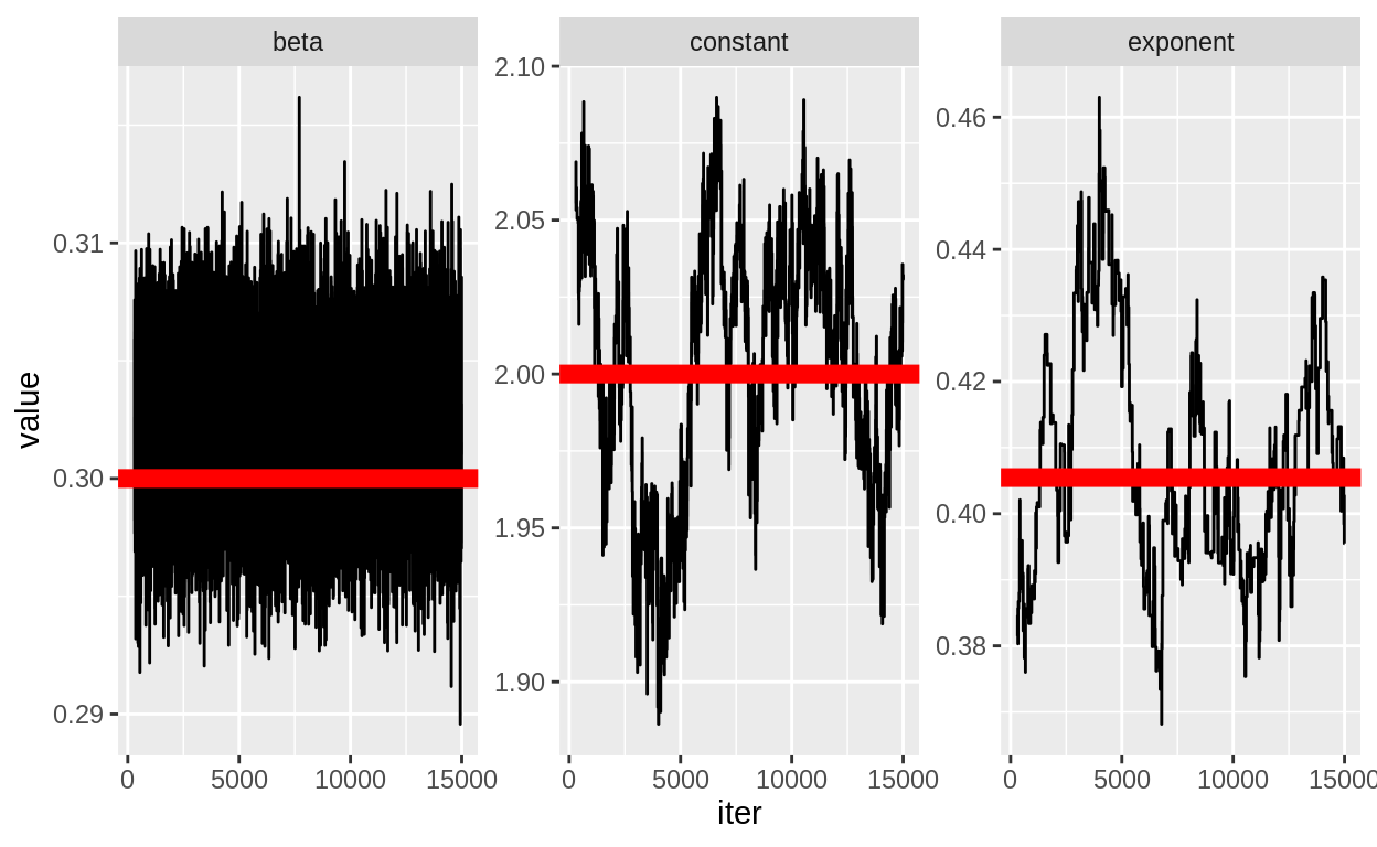
Here are a few thoughts on this process:

samplers are rather sensitive to things like starting values, tuning parameters, prior choice, model structure etc. What adjustments could you make to this to improve the algorithm?
I chose a VERY large sample size because I want to think about the algorithm itself. What happens if we choose a more realistic sample size?

Posterior plots to check your model

We don’t have space in this already LONG document to cover the whole story of how to work with a posterior distribution. This includes things like: * making predictions to see if your model is working well * plotting averages or regression lines * making predictions for the results of some manipulation (future projection, adding or removing a treatment) * calculating quantities of interest to look at their values (e.g. is the difference between two groups large or small? how sure are we?)

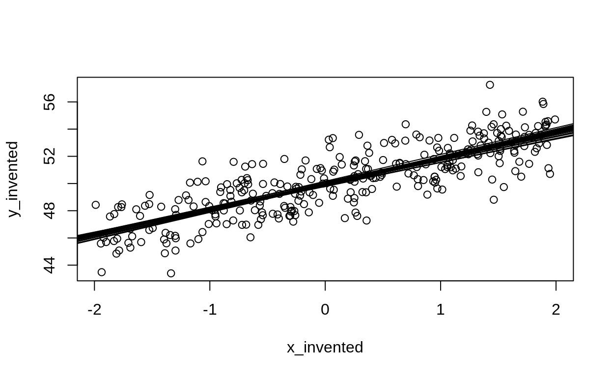
But I do want to show one quick thing we can do with this model: let’s plot the average line, aka the “fitted” values. This shows us what kinds of curvy lines the model thinks are “reasonable”.

gibbs_df <- gibbs_chain %>% as_tibble() %>% 
  mutate(iter = 1:n_iter)

with(energy_mass, plot(masses, energies))

gibbs_df %>% 
  filter(iter > (n_iter-300)) %>% 
  sample_n(20) %>% 
  transpose %>% 
  walk(~ lines(x = 0:310, 
               y = .$constant*(0:310)^plogis(.$exponent),
               col = "red"))

The lines are reasonably close to the true values (though not quite) and the plot looks pretty good.

Bonus Zone

some more material that I either cut, streamlined, or didn’t have the time to get to! enjoy if you like :)

Conjugate priors, Metropolis-Hastings, and Penguins

Proof of Beta & Binomial conjugate pair

\[ \begin{align} [p|\text{trials}, \text{successes}, \alpha, \beta] &\propto [\text{successes} | \text{trials}, p] \times [p | \alpha , \beta]\\ &\propto \text{Binomial}(p,\text{trials}) \times \text{Beta}(\alpha, \beta)\\ &\propto{\text{trials} \choose \text{successes}}p^\text{successes}(1-p)^{\text{trials}-\text{successes}} \times \text{B} p^{\alpha - 1}(1-p)^{\beta - 1}\\ &\propto p^\text{successes}(1-p)^{\text{trials}-\text{successes}} \times p^{\alpha - 1}(1-p)^{\beta - 1}\\ &\propto p^{\alpha + \text{successes} - 1}(1-p)^{ \beta + \text{trials}-\text{successes} - 1} \end{align} \]

Now we only have to realize that the last line is a beta distribution, without the magic number that we called “\(B\)” before. This value is what’s called a “normalizing constant”. Normalizing constants make the proportional expression (like the one above) into a probability distribution

\[ [p|\text{trials}, \text{successes}, \alpha, \beta] = \text{Beta}(\alpha + \text{successes} - 1, \beta + \text{trials}-\text{successes} - 1) \]

So the posterior distribution is a Beta distribution, just like the prior was! We have it already, with no need for any fancy sampling approach.

This also gives us an easy interpretation of what the parameters of any Beta distribution are: \(\alpha\) is something like the number of successes, and \(\beta\) is something like the number of failures⁶.

Suppose we had written the model like this:

\[ \begin{align} y &\sim \text{Binomial}(p, N) \\ \text{logit}(p) &= \alpha\\ \alpha &\sim \text{Normal}(1, 1) \end{align} \]

Remember that the binomial distribution is written as:

\[ {n \choose k} p^k (1-p)^{n-k} \]

the two lines in equation 1 are just a shorthand for saying “replace \(p\) with the inverse logit of \(\alpha\)”. We could also write it this way, literally replacing \(p\) with that function

\[ \begin{align} y &\sim {n \choose k} \left(\frac{e^\alpha}{1 + e^\alpha} \right)^{k}\left(1-\frac{e^\alpha}{1 + e^\alpha}\right)^{n-k} \\ \alpha &\sim \text{Normal}(1, 1) \end{align} \]

Another quick reminder, remember that the logistic function is a traditional way of squishing any real number into the interval \((0,1)\):

\[ \frac{e^x}{1 + e^x} \]

curve(exp(x)/(1 + exp(x)),
      xlim = c(-4, 4), ylim = c(0, 1))

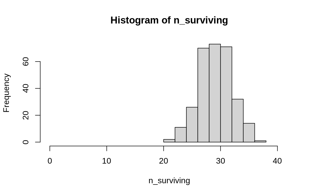
Let’s imagine an experiment where we place exactly 42 seeds in experimental plots. We use 30 experimental plots.

We want to estimate a probability of germination for these seedlings

Our model looks like this:

\[ \begin{align} y &\sim \text{Binomial}(p_{\text{survival}}, 42)\\ p_{\text{survival}} &\sim \text{Beta}(2,5)\\ \end{align} \]

in English, this means:

We thing that the number of seedlings which germinate will follow a Binomial distribution. This means that out of a total of 42, some survive. The probability for any surviving is the same: \(p_{\text{survival}}\)

## start with some survival data -- out of 42
true_prob <- 0.7

set.seed(1859)
n_surviving <- rbinom(n = 300, size = 42, prob = true_prob)

hist(n_surviving, xlim = c(0, 42))

Can use the conjugate posterior.

First, use the conjugate prior to the binomial (beta distribution).

curve(dbeta(x, 2,5))

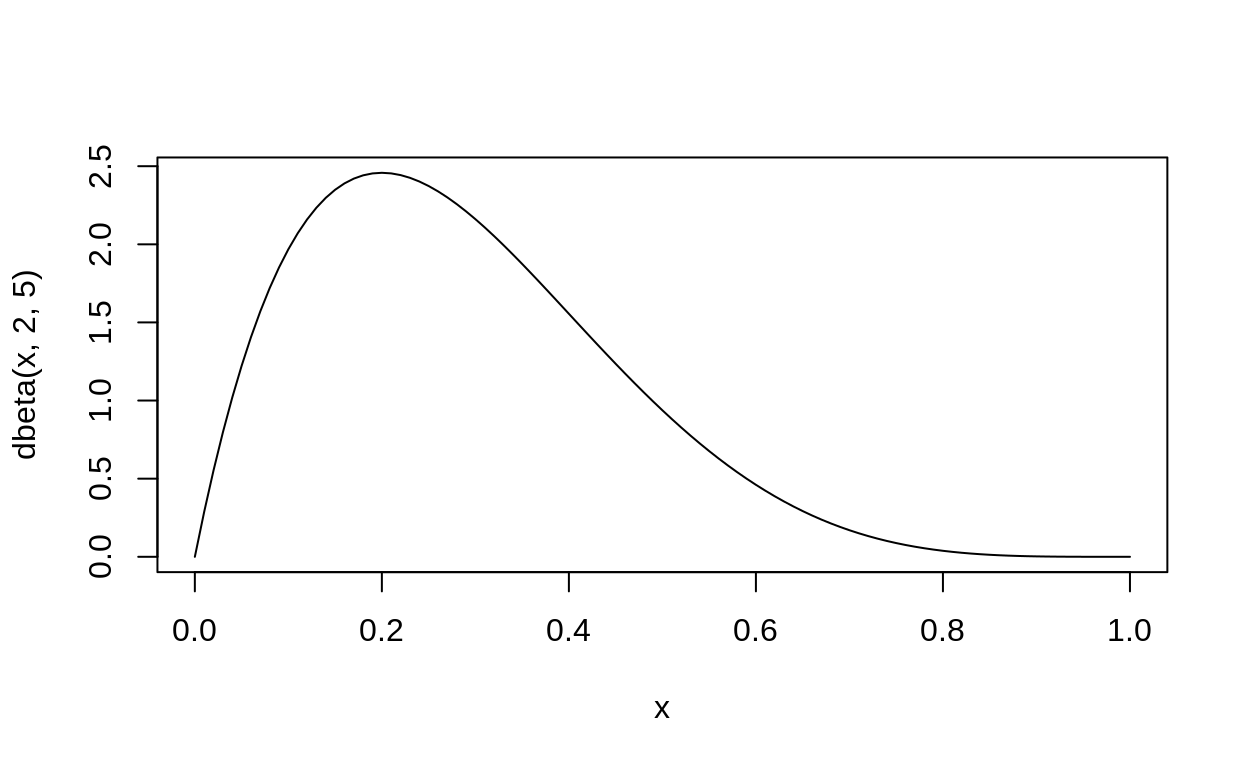
This might be a reasonable first guess. But what does it actually mean? we need to do predictions to make sure.

possible_probabilities <- rbeta(300, 2, 5)

hist(rbinom(30, 42, possible_probabilities), xlim = c(0, 42))

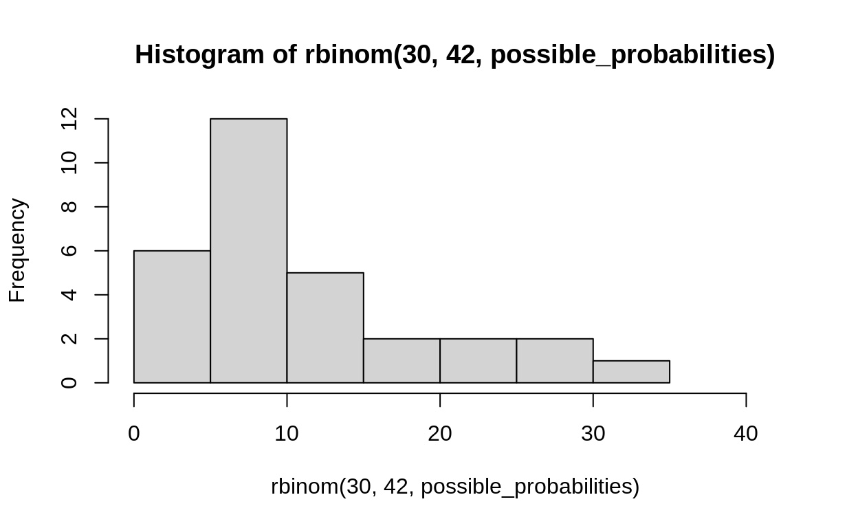
Do this a bunch of times, to see if the prior is foolish or not.

With enough data, even an outlandish prior is fine:

lived <- sum(n_surviving)
died <- sum(42 - n_surviving)

calculate the posterior

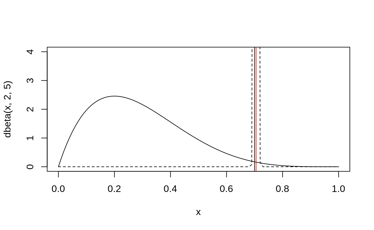
curve(dbeta(x, 2, 5),ylim = c(0,4))
curve(dbeta(x, 2 + lived, 5 + died), add = TRUE, lty = 2)
abline(v = true_prob)

abline(v =(2 + lived)/(2 + lived + 5 + died), col = "red")

Sampling this model: the Metropolis algorithm

Once again, our model is:

\[ \begin{align} y &\sim \text{Binomial}(p, N) \\ \text{logit}(p) &= \alpha\\ \alpha &\sim \text{Normal}(1, 1) \end{align} \]

Now we have no conjugate posterior for \(\alpha\). However, just because we can’t calculate the distribution doesn’t mean we can’t sample it!

We can use the Metropolis algorithm.

## define likelihoods for our problem
binomial_loglike <- function(data_vec, prob_new){
  sum(dbinom(data_vec, size = 42, 
             prob = prob_new, log = TRUE))
}

normal_loglike <- function(val, mean_prior, sd_prior){
  dnorm(val, mean = mean_prior, sd = sd_prior, log = TRUE)
}


# define our function
logistic_curve <- function(x) exp(x)/(1 + exp(x))

## function to use these to calculate the value of the numerator in Bayes Formula
numerator <- function(v, data)  {
  binomial_loglike(data_vec = data, prob_new = logistic_curve(v)) + 
    normal_loglike(val = v, mean = -1, sd = 2)
}

## function to calculate the acceptance ratio
accept_probability <- function(new_value, old_value, data_to_use) {
  r <- exp(numerator(v = new_value, data = data_to_use) - 
        numerator(v = old_value, data = data_to_use))
  
  p_accept <- min(1, r)
  
  return(p_accept)
}

# proposal function to make new parameter values.
propose_new <- function(x, sig_tune) rnorm(1, mean = x, sd = sig_tune)

# start value
metropolis <- function(dataset,
                       n_samples,
                       tune_parameter,
                       start_value){
  chain <- numeric(n_samples)
  
  chain[1] <- start_value
  
  for (i in 2:length(chain)) {
    
    old <- chain[i - 1]
    
    new <- propose_new(old, sig_tune = tune_parameter)
    
    p_accept <- accept_probability(new_value = new,
                                   old_value = old, 
                                   data_to_use = dataset)
    
    chain[i] <- ifelse(runif(1) < p_accept, new, old)
  }
  return(chain)
}


chain <- metropolis(dataset = n_surviving,
                    n_samples = 3000,
                    tune_parameter = 0.2, 
                    start_value = 0)

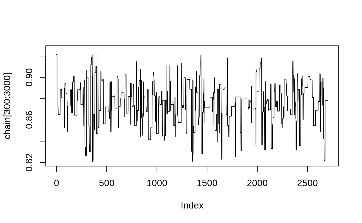
plot(chain[300:3000], type = "l")

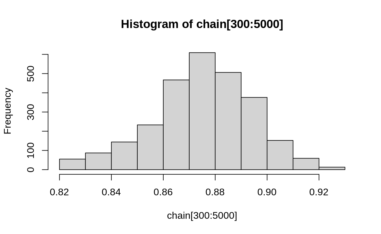
hist(chain[300:5000])

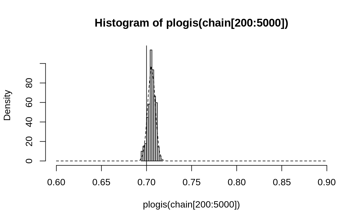
hist(plogis(chain[200:5000]), xlim = c(0.6,.9), probability = TRUE)
abline(v = true_prob)

curve(dbeta(x, 2 + lived, 5 + died), add = TRUE, lty = 2)

Application: Clutch success in the Palmer Penguins

pr <- read.csv(path_to_file("penguins_raw.csv"))
penguins_raw %>% 
  count(Species, `Clutch Completion`) %>% 
  pivot_wider(names_from = `Clutch Completion`, values_from = n) %>% 
  knitr::kable(.)

Species	No	Yes
Adelie Penguin (Pygoscelis adeliae)	14	138
Chinstrap penguin (Pygoscelis antarctica)	14	54
Gentoo penguin (Pygoscelis papua)	8	116

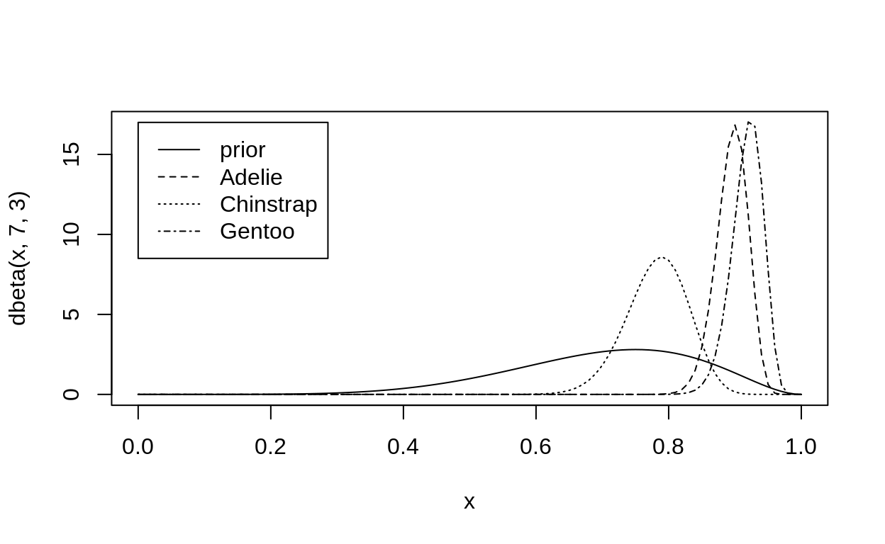
With this, we can calculate the posterior probability of clutch success for each penguin species.

\[ \begin{align} n_{\text{succeeded}} &\sim \text{Binomial}(p_{\text{success}}, n_{\text{nesting}})\\ p_{\text{success}} &\sim \text{Beta}(7,3)\\ \end{align} \]

curve(dbeta(x, 7, 3), ylim = c(0, 17))
curve(dbeta(x, 138 + 7, 14 + 3), add = TRUE, lty = 2)
curve(dbeta(x, 54 + 7, 14 + 3), add = TRUE, lty = 3)
curve(dbeta(x, 116 + 7, 8 + 3), add = TRUE, lty = 4)
legend(0,17, legend = c("prior", "Adelie", "Chinstrap", "Gentoo"), lty = 1:4)

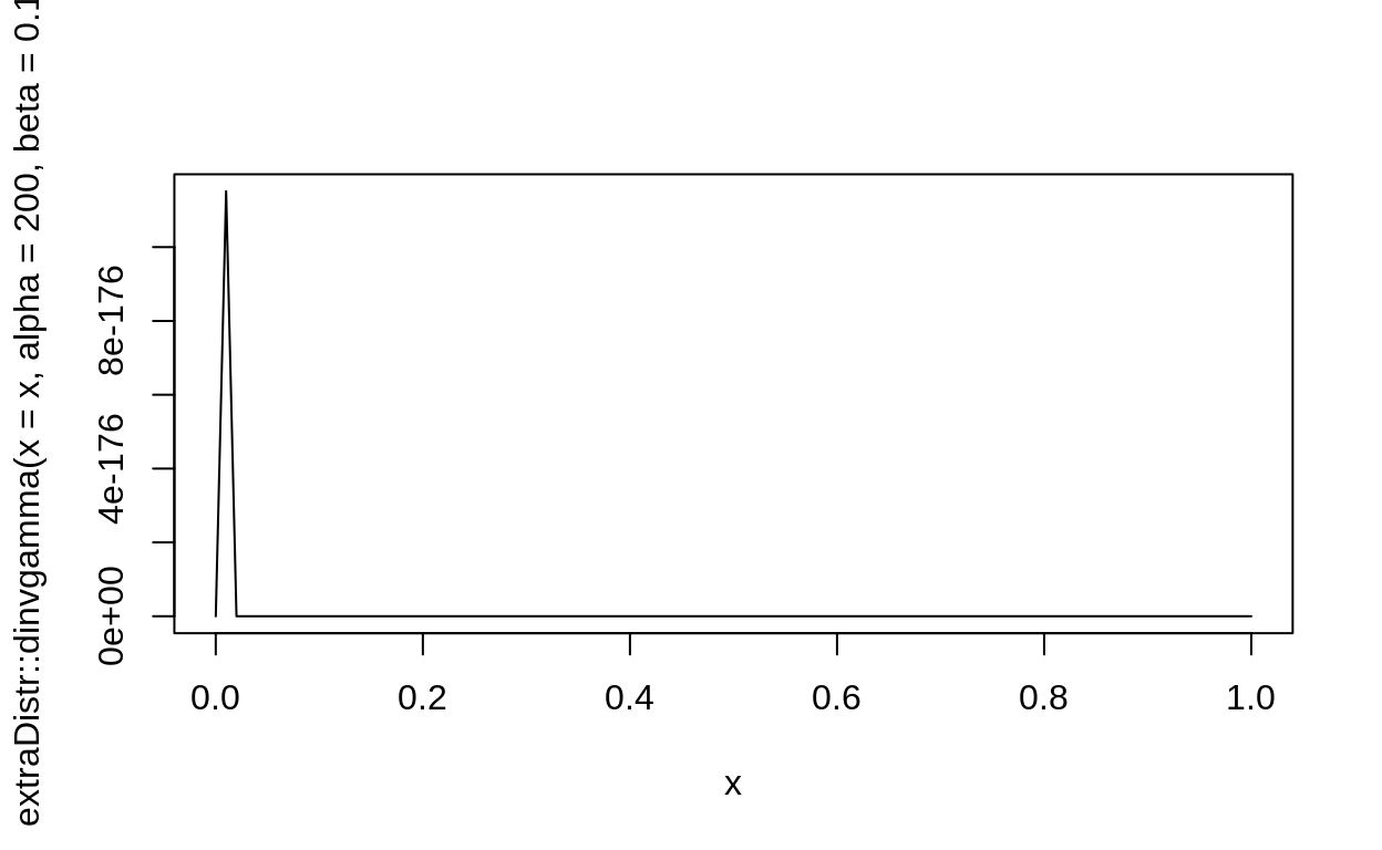
Exploring the Inverse Gamma

Here is a quick simulation to demonstrate (explore on your own if you want!):

# constant mean
truemean <- 60
sig <- .6

ff <- rlnorm(1000,
             meanlog = log(truemean), 
             sdlog = sig)

ff %>% median

sd(ff)

curve(extraDistr::dinvgamma(x, 
                            alpha = 3 + length(ff)/2,
                            beta = 4 + sum( (log(ff) - log(truemean))^2 ) / 2),
      xlim = c(0,1)
      # add = TRUE
)
abline(v = sig^2, col = "red")

## moving mean

x <- runif(1000, 0, 3)

truemean2 <- x*3

ff2 <- rlnorm(1000,
             meanlog = log(truemean), 
             sdlog = sig)

plot(x, ff2)

curve(extraDistr::dinvgamma(x, 
                            alpha = 3 + length(ff2)/2,
                            beta = 4 + sum( (log(ff2) - log(truemean2))^2 ) / 2),
      xlim = c(0,1)
      # add = TRUE
)

abline(v = sig^2, col = "red")

# nonlinear
truemean3 <- 3*x^.7

ff3 <- rlnorm(1000,
             meanlog = log(truemean3), 
             sdlog = sig)

plot(x, ff3)


curve(extraDistr::dinvgamma(x, 
                            alpha = 3 + length(ff3)/2,
                            beta = 4 + sum( (log(ff3) - log(truemean3))^2 ) / 2),
      xlim = c(0,1)
      # add = TRUE
)

abline(v = sig^2, col = "red")

quick demo: if we knew the real values what would this mean:

true_beta <- .3
true_constant <-  2
true_exponent <- .6
sample_size <- 1000
set.seed(1859)

energy_mass <- tibble(
  masses = runif(n = sample_size, min = 2, max = 320),
  median_energy = true_constant * masses^true_exponent,
  energies = rlnorm(n = sample_size,
                    meanlog = log(median_energy), 
                    sdlog = true_beta))

data_figure <- energy_mass %>% 
  ggplot(aes(x = masses, y = energies)) + geom_point()
data_figure

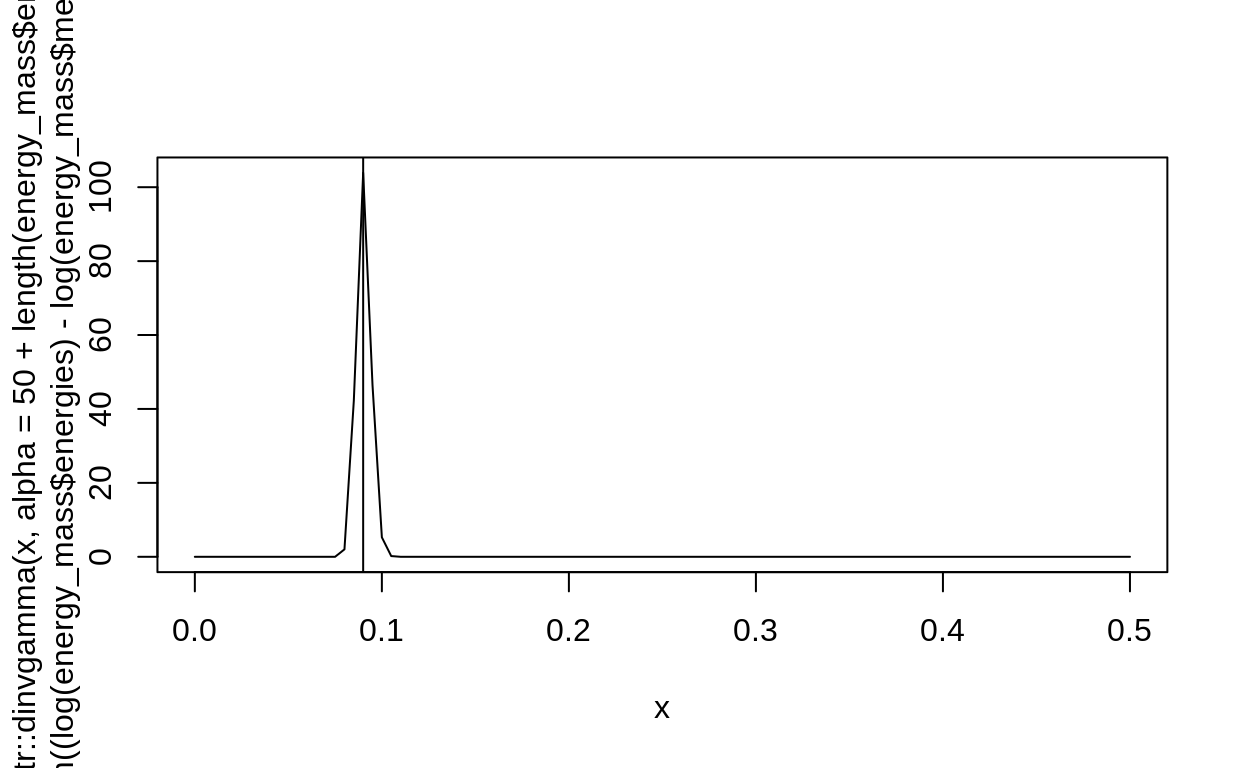
curve(extraDistr::dinvgamma(x, 
                            alpha = 50 + length(energy_mass$energies)/2,
                            beta = 4 + sum( (log(energy_mass$energies) - log(energy_mass$median_energy))^2 ) / 2),
      xlim = c(0.,.5)
      # add = TRUE
)

abline(v = true_beta^2)

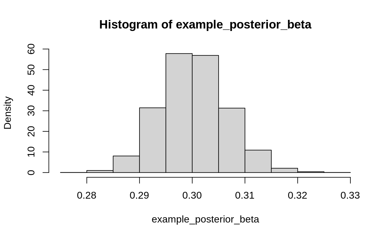
example_posterior_beta <- replicate(4000,
          sample_beta(y = energy_mass$energies,
                      alpha = calculate_alpha(
                        constant = true_constant,
                        logit_exponent = qlogis(true_exponent),
                        mass_data = energy_mass$masses)
            )
)

hist(example_posterior_beta, probability = TRUE)

abline(v = true_beta^2, col = "red")

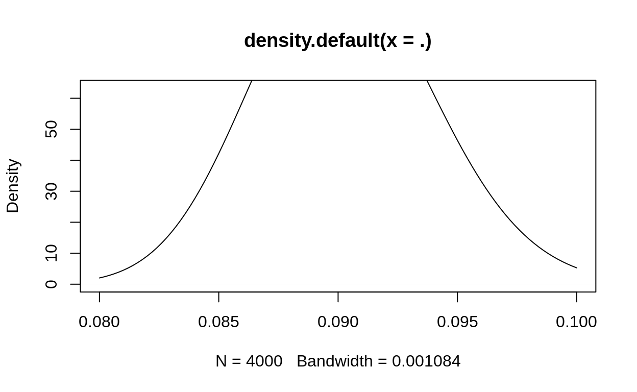
example_posterior_beta %>% density %>% plot(xlim = c(0.08,.1))

curve(extraDistr::dinvgamma(x, 
                            alpha = 50 + length(energy_mass$energies)/2,
                            beta = 4 + sum( (log(energy_mass$energies) - log(energy_mass$median_energy))^2 ) / 2),
      xlim = c(0.08,.1),
      add = TRUE
)

hist(example_posterior_beta %>% sqrt)


abline(v = true_beta, col = "red")

Three parameters at once

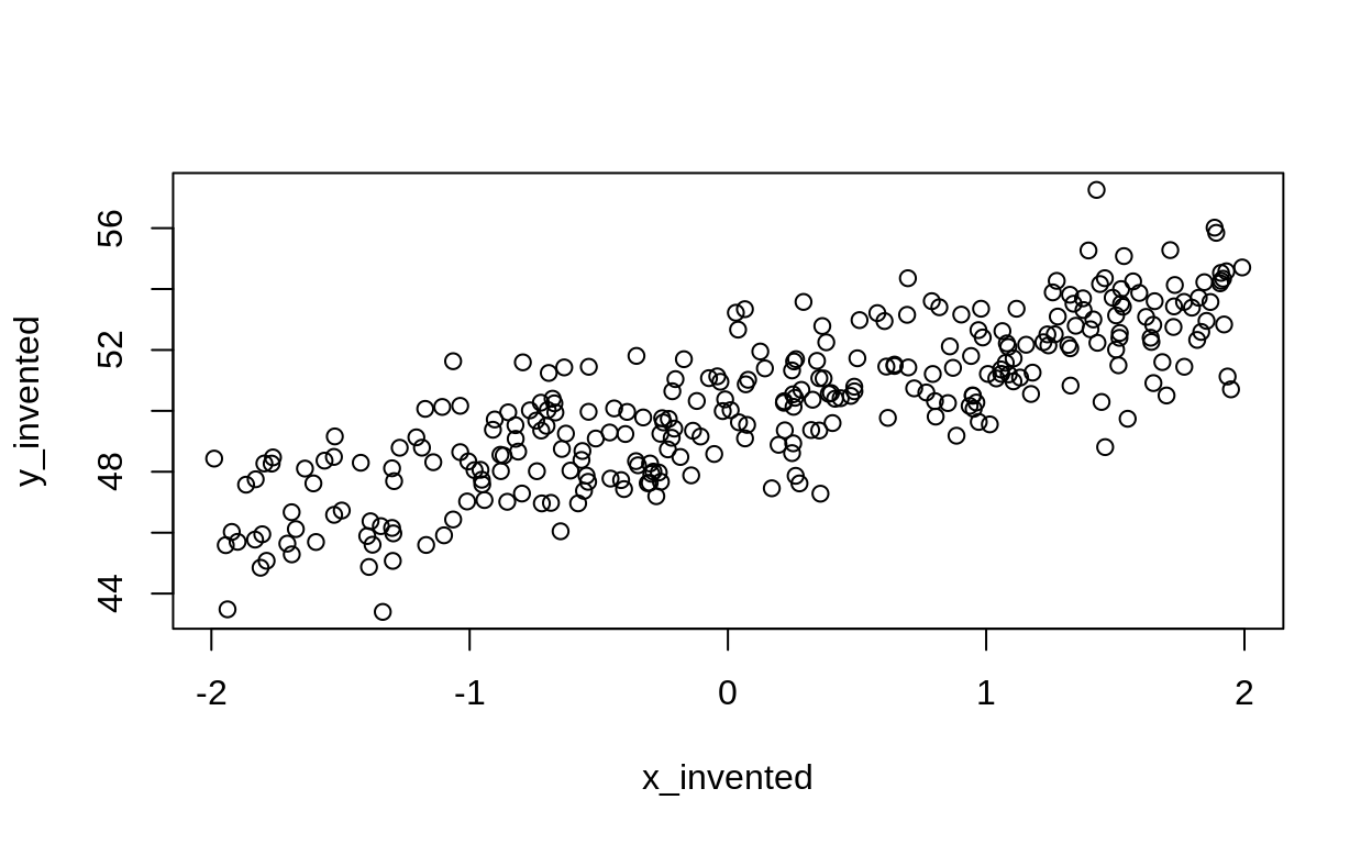
Imagine that you are doing a simple linear regression and you want to get three parameters: the slope, the intercept, and the variance of the observations.

We perform the same procedure, looking for gibbs samples where we can.

n_invented <- 300
x_invented <- runif(n = n_invented, -2, 2) 

true_intercept <- 50
true_slope <- 2

true_observation_sd <- 1.5

y_invented <- rnorm(n = n_invented, 
                    mean = true_intercept + true_slope*x_invented, 
                    sd = true_observation_sd)

plot(x_invented, y_invented)

# gibbs process
n_iterations <- 2000
b0_chain <- numeric(n_iterations)
b1_chain <- numeric(n_iterations)
observation_sd_chain <- numeric(n_iterations)


# sample to start -- could be anything, might as well be priors
b0_chain[1] <- rnorm(1, mean = 10, sd = 5)
b1_chain[1] <- rnorm(1, mean = 0, sd = 2)
observation_sd_chain[1] <- rgamma(1, shape = 3^2/2^2, rate = 3/2^2)

for (k in 2:n_iterations) {
  # draw a mean
  b0_chain[k] <- post_mean(
    y_vector = y_invented - x_invented * b1_chain[k - 1],
    known_sigma = observation_sd_chain[k - 1],
    prior_mean = 10,
    prior_sd = 5)
  b1_chain[k] <- post_mean(
    y_vector = (y_invented - b0_chain[k])*x_invented,
    known_sigma = observation_sd_chain[k - 1],
    prior_mean = 0,
    prior_sd = 2, 
    n = sum(x_invented^2))
  observation_sd_chain[k] <- post_sd(
    y_vector = y_invented, 
    known_mean = b0_chain[k] + x_invented * b1_chain[k],
    prior_alpha = 3^2/2^2,
    prior_beta = 3/2^2)
}

par(mfrow = c(1,3))
plot(b0_chain[100:n_iterations])
abline(h = true_intercept, col = "red", lwd = 2)
plot(b1_chain[100:n_iterations])
abline(h = true_slope, col = "red", lwd = 2)
plot(observation_sd_chain[100:n_iterations])
abline(h = true_observation_sd, col = "red", lwd = 2)

par(mfrow = c(1,1))

# plot these regression lines

plot(x_invented, y_invented)

for (k in 200:220){
  abline(a = b0_chain[k], b = b1_chain[k])
}

could also plot some interesting posterior predictive plots in this way.

Metropolis hastings and gibbs at the same time

Sometimes you will have a model for which you can’t (or don’t want to) use conjugate posteriors for each of the conditional distributions.

Clara Coffee Example

clara_coffee <- tibble::tribble(
  ~Coffee_extraction, ~time,
  15.88,              19.13875598,
  16.72,              7.633587786,
  16.72,              22.90076336,
  17,                       30,
  17.3,              5.479452055,
  17.64,              12.93103448,
  17.75,              9.459459459,
  17.77,              12.93103448,
  17.99,              10.18867925,
  18,                        6,
  18.03,              11.86440678,
  18.32,              15.54404145,
  18.57,              23.71794872,
  18.89,              24.75247525,
  19.13,                      6.4,
  19.33,              20.30456853,
  19.36,              18.71345029,
  19.5,              33.49282297,
  19.67,              13.61867704,
  20.23,              15.81027668,
  20.26,              17.54385965,
  20.39,              13.76146789,
  20.45,              14.93775934,
  20.57,              13.61867704,
  20.61,              14.85148515,
  20.69,                39.408867,
  20.76,              6.944444444,
  20.84,              8.968609865,
  20.88,              11.40684411,
  20.95,              9.756097561,
  21.04,              4.843304843,
  21.2,               14.0969163,
  21.25,                     15.2,
  21.36,              6.060606061,
  21.72,              11.52073733,
  21.86,              10.89494163,
  22.14,              8.849557522,
  22.26,              8.532423208,
  22.47,              13.39285714,
  22.48,              5.333333333,
  23.48,              6.134969325,
  24.29,              6.993006993,
  24.35,               7.86163522,
  24.63,              12.95336788
)


library(ggplot2)

ggplot(clara_coffee, aes(x = time, y = Coffee_extraction/100)) +
  geom_point()

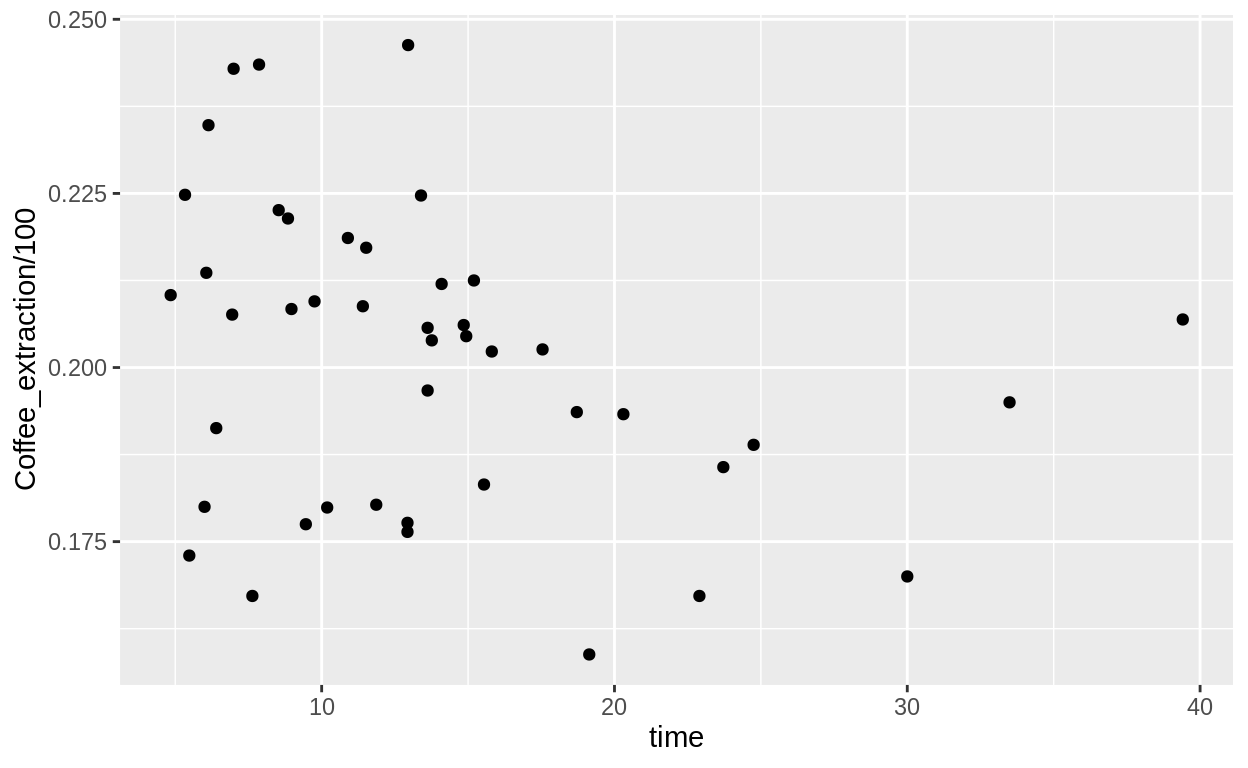
#' what are the response distribution?
#'
#' what is the question?

#' quel est la relation entre la coulée d'eau et lextraction de cafe
#'

# response distribtuion -- between 0 and 1. Could be the beta.

# normal -- for pragmatic reasons ?

curve(dgamma(x, shape = (2)^2/4, rate = 2/4), xlim = c(0,5))

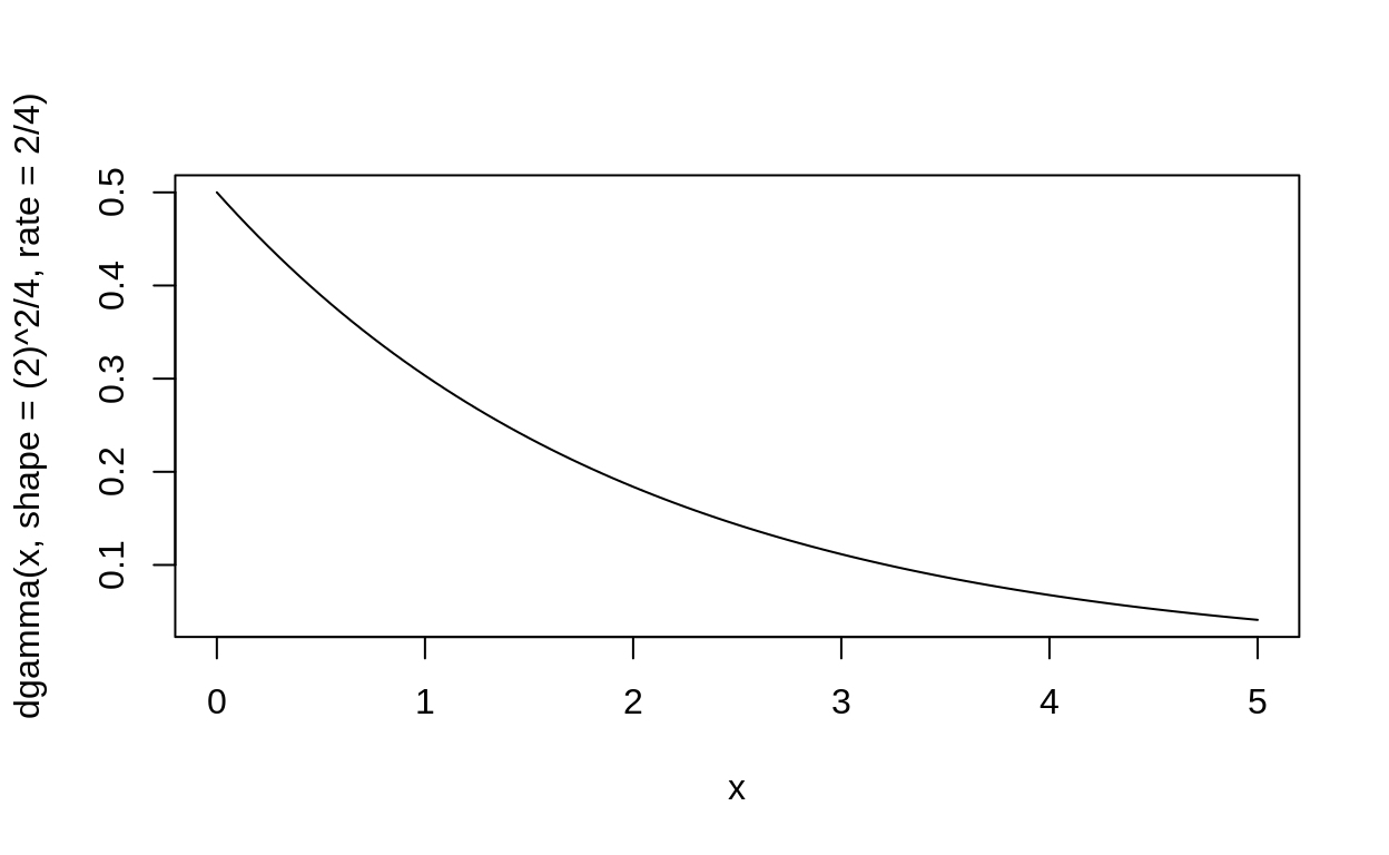
sigma_coffee <- 1/sqrt(rgamma(1, shape = (2)^2/4, rate = 2/4))
mean_coffee <- rnorm(1, 21, 3)
change_coffee <- rnorm(1, 1, 1)

clara_coffee$t_centered <- with(clara_coffee, time - mean(time))

clara_coffee_prior <- transform(clara_coffee,
                                average_measure = mean_coffee +
                                  change_coffee*t_centered)

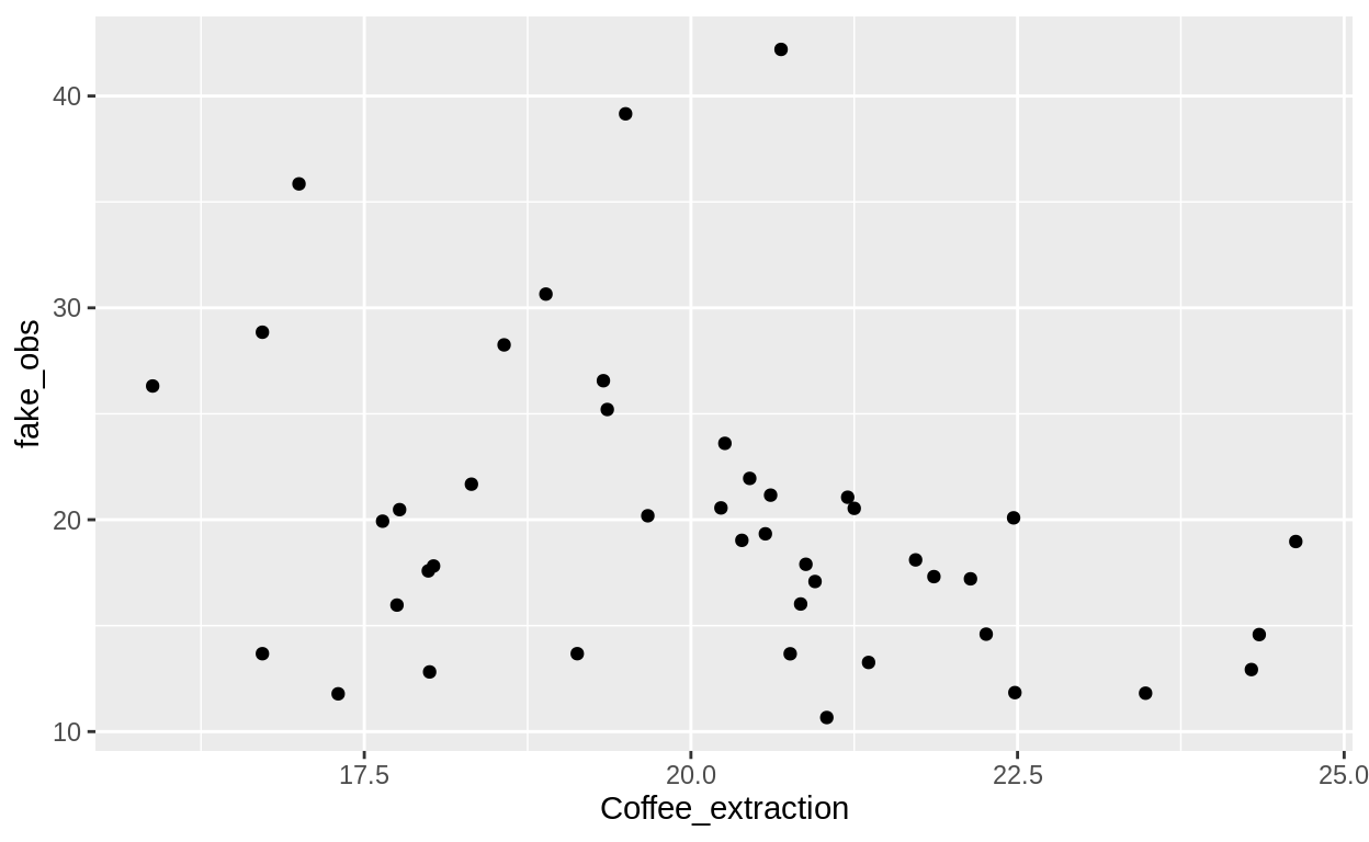
clara_coffee_prior$fake_obs <- rnorm(n = nrow(clara_coffee),
                                     mean = clara_coffee_prior$average_measure,
                                     sd = sigma_coffee)


ggplot(clara_coffee_prior, aes(x = Coffee_extraction, y = fake_obs)) +
  geom_point()

library(brms)

coffee_formula <- bf(Coffee_extraction ~ t_centered)

get_prior(coffee_formula, data = clara_coffee_prior)

cafe_stan <- brm(Coffee_extraction ~ t_centered,
                     data = clara_coffee_prior, )

except for the Normal distribution. The Normal is a beautiful weirdo which is why we love it!↩︎
Why do we do the inverse square? Well, the square of the standard deviation is the variance. As we know, the larger the variance, the wider the distribution. The inverse variance has the opposite interpretation: the larger it is, the more narrow and focussed the distribution! This is called the “precision”, and it is another common way to think about the Normal Distribution.↩︎
Conjugate priors are not automatically GOOD priors – either in terms of the behaviour of the model or in terms of what they mean biologically. Modern methods for estimating the posterior, such as Stan, don’t have this restriction.↩︎
This is a classic result in Ecology! However I’ve only taken care to match the qualitative shape of this relationship, not the real units. If you have improvements to suggest please message me!↩︎
quick reminder that using the logit link is a conventional way to take any real number and squish it into the interval \((0,1)\). This means we will be taking values from a normal distribution and feeding them through the inverse logit function to get the value for \(b\) in the equation. In other words, if \(x \sim \text{Normal}(0,1)\) then \(b = \frac{e^x}{1 + e^x}\)↩︎
Not EXACTLY successes and failures because \(\alpha\) and \(\beta\) can be decimal numbers (e.g. “1.5”) and obviously real successes and failures can’t be. You can think of these as “pseudosuccesses” and “pseudofailures” or, as I prefer, “successosity” and “failishness” ↩︎